Báo cáo khoa học: "Why Initialization Matters for IBM Model 1: Multiple Optima and Non-Strict Convexity" pptx
Bạn đang xem bản rút gọn của tài liệu. Xem và tải ngay bản đầy đủ của tài liệu tại đây (202.76 KB, 6 trang )
Proceedings of the 49th Annual Meeting of the Association for Computational Linguistics:shortpapers, pages 461–466,
Portland, Oregon, June 19-24, 2011.
c
2011 Association for Computational Linguistics
Why Initialization Matters for IBM Model 1:
Multiple Optima and Non-Strict Convexity
Kristina Toutanova
Microsoft Research
Redmond, WA 98005, USA
Michel Galley
Microsoft Research
Redmond, WA 98005, USA
Abstract
Contrary to popular belief, we show that the
optimal parameters for IBM Model 1 are not
unique. We demonstrate that, for a large
class of words, IBM Model 1 is indifferent
among a continuum of ways to allocate prob-
ability mass to their translations. We study the
magnitude of the variance in optimal model
parameters using a linear programming ap-
proach as well as multiple random trials, and
demonstrate that it results in variance in test
set log-likelihood and alignment error rate.
1 Introduction
Statistical alignment models have become widely
used in machine translation, question answering,
textual entailment, and non-NLP application areas
such as information retrieval (Berger and Lafferty,
1999) and object recognition (Duygulu et al., 2002).
The complexity of the probabilistic models
needed to explain the hidden correspondence among
words has necessitated the development of highly
non-convex and difficult to optimize models, such
as HMMs (Vogel et al., 1996) and IBM Models 3
and higher (Brown et al., 1993). To reduce the im-
pact of getting stuck in bad local optima the orig-
inal IBM paper (Brown et al., 1993) proposed the
idea of training a sequence of models from simpler
to complex, and using the simpler models to initial-
ize the more complex ones. IBM Model 1 was the
first model in this sequence and was considered a
reliable initializer due to its convexity.
In this paper we show that although IBM Model 1
is convex, it is not strictly convex, and there is a large
space of parameter values that achieve the same op-
timal value of the objective.
We study the magnitude of this problem by for-
mulating the space of optimal parameters as solu-
tions to a set of linear equalities and seek maximally
different parameter values that reach the same objec-
tive, using a linear programming approach. This lets
us quantify the percentage of model parameters that
are not uniquely defined, as well as the number of
word types that have uncertain translation probabil-
ities. We additionally study the achieved variance in
parameters resulting from different random initial-
ization in EM, and the impact of initialization on test
set log-likelihood and alignment error rate. These
experiments suggest that initialization does matter
in practice, contrary to what is suggested in (Brown
et al., 1993, p. 273).
1
2 Preliminaries
In Appendix A we define convexity and strict con-
vexity of functions following (Boyd and Vanden-
berghe, 2004). In this section we detail the gener-
ative model for Model 1.
2.1 IBM Model 1
IBM Model 1 (Brown et al., 1993) defines a genera-
tive process for a source sentences f = f
1
. . . f
m
and
alignments a = a
1
. . . a
m
given a corresponding tar-
get translation e = e
0
. . . e
l
. The generative process
is as follows: (i) pick a length m using a uniform
distribution with mass function proportional to ; (ii)
for each source word position j, pick an alignment
1
When referring to Model 1, Brown et al. (1993) state that
“details of our initial guesses for t(f|e) are unimportant”.
461
position in the target sentence a
j
∈ 0, 1, . . . , l from
a uniform distribution; and (iii) generate a source
word using the translation probability distribution
t(f
j
|e
a
j
). A special empty word (NULL) is assumed
to be part of the target vocabulary and to occupy
the first position in each target language sentence
(e
0
=NULL).
The trainable parameters of Model 1 are the lex-
ical translation probabilities t(f |e), where f and e
range over the source and target vocabularies, re-
spectively. The log-probability of a single source
sentence f given its corresponding target sentence e
and values for the translation parameters t(f |e) can
be written as follows (Brown et al., 1993):
m
j=1
log
l
i=0
t(f
j
|e
i
) − m log (l + 1) + log
The parameters of IBM Model 1 are usu-
ally derived via maximum likelihood estimation
from a corpus, which is equivalent to negative
log-likelihood minimization. The negative log-
likelihood for a parallel corpus D is:
L
D
(T ) = −
f ,e
m
j=1
log
l
i=0
t(f
j
|e
i
) + B (1)
where T is the matrix of translation probabilities
and B represents the other terms of Model 1 (string
length probability and alignment probability), which
are constant with respect to the translation parame-
ters t(f|e).
We can define the optimization problem as the
one of minimizing negative log-likelihood L
D
(T )
subject to constraints ensuring that the parameters
are well-formed probabilities, i.e., that they are non-
negative and summing to one. It is well-known that
the EM algorithm for this problem converges to a lo-
cal optimum of the objective function (Dempster et
al., 1977).
3 Convexity analysis for IBM Model 1
In this section we show that, contrary to the claim in
(Brown et al., 1993), the optimization problem for
IBM Model 1 is not strictly convex, which means
that there could be multiple parameter settings that
achieve the same globally optimal value of the ob-
jective.
2
The function − log(x) is strictly convex (Boyd
and Vandenberghe, 2004). Each term in the nega-
tive log-likelihood is a negative logarithm of a sum
of parameters. The negative logarithm of a sum is
not strictly convex, as illustrated by the following
simple counterexample. Let’s look at the function
− log(x
1
+ x
2
). We can express it in vector notation
using − log(1
T
x), where 1 is a vector with all ele-
ments equal to 1. We will come up with two param-
eter settings x,y and a value θ that violate the defini-
tion of strict convexity. Take x = [x
1
, x
2
] = [.1, .2],
y = [y
1
, y
2
] = [.2, .1] and θ = .5. We have
z = θx + (1 − θ)y = [z
1
, z
2
] = [.15, .15]. Also
− log(1
T
(θx + (1 − θ)y)) = − log(z
1
+ z
2
) =
− log(.3). On the other hand, −θ log(x
1
+ x
2
) −
(1−θ) log(y
1
+y
2
) = − log(.3). Strict convexity re-
quires that the former expression be strictly smaller
than the latter, but we have equality. Therefore, this
function is not strictly convex. It is however con-
vex as stated in (Brown et al., 1993), because it is a
composition of log and a linear function.
We thus showed that every term in the negative
log-likelihood objective is convex but not strictly
convex and thus the overall objective is convex, but
not strictly convex. Because the objective is con-
vex, the inequality constraints are convex, and the
equality constraints are affine, the IBM Model 1 op-
timization problem is a convex optimization prob-
lem. Therefore every local optimum is a global op-
timum. But since the objective is not strictly con-
vex, there might be multiple distinct parameter val-
ues achieving the same optimal value. In the next
section we study the actual space of optima for small
and realistically-sized parallel corpora.
2
Brown et al. (1993, p. 303) claim the following about
the log-likelihood function (Eq. 51 and 74 in their paper, and
Eq. 1 in ours): “The objective function (51) for this model is a
strictly concave function of the parameters”, which is equivalent
to claiming that the negative log-likelihood function is strictly
convex. In this section, we will theoretically demonstrate that
Brown et al.’s claim is in fact incorrect. Furthermore, we will
empirically show in Sections 4 and 5 that multiple distinct pa-
rameter values can achieve the global optimum of the objective
function, which also disproves Brown et al.’s claim about the
strict convexity of the objective function. Indeed, if a function
is strictly convex, it admits a unique globally optimum solution
(Boyd and Vandenberghe, 2004, p. 151), so our experiments
prove by modus tollens that Brown et al.’s claim is wrong.
462
4 Solution Space
In this section, we characterize the set of parameters
that achieve the maximum of the log-likelihood of
IBM Model 1. As illustrated with the following
simple example, it is relatively easy to establish
cases where the set of optimal parameters t(f |e) is
not unique:
e : short sentence f : phrase courte
If the above sentence pair represents the entire
training data, Model 1 likelihood (ignoring NULL
words) is proportional to
t(phrase|shor t) + t(phrase|sentence)
·
t(courte|short) + t(courte|sentence)
which can be maximized in infinitely many differ-
ent ways. For instance, setting t(phrase|sentence) =
t(courte|short) = 1 yields the maximum likelihood
value with (0 + 1)(1 + 0) = 1, but the most
divergent set of parameters (t(courte|sentence) =
t(phrase|sentence) = 1) also reaches the same op-
timum: (1+0)(0+1) = 1. While this example may
not seem representative given the small size of this
data, the laxity of Model 1 that we observe in this
example also surfaces in real and much larger train-
ing sets. Indeed, it suffices that a given pair of target
words (e
1
,e
2
) systematically co-occurs in the data
(as with e
1
= short e
2
= sentence) to cause Model 1
to fail to distinguish the two.
3
To characterize the solution space, we use the def-
inition of IBM Model 1 log-likelihood from Eq. 1 in
Section 2.1. We ask whether distinct sets of parame-
ters yield the same minimum negative log-likelihood
value of Eq. 1, i.e., whether we can find distinct
models t(f|e) and t
(f|e) so that:
f ,e
m
j=1
log
l
i=0
t(f
j
|e
i
) =
f ,e
m
j=1
log
l
i=0
t
(f
j
|e
i
)
Since the negative logarithm is strictly convex, the
3
Since e
1
and e
2
co-occur with exactly the same source
words, one can redistribute the probability mass between
t(f|e
1
) and t(f|e
2
) without affecting the log-likelihood.
This is true if (a) the two distributions remain well-formed:
j
t(f
j
|e
i
) = 1 for i ∈ {1, 2}; (b) any adjustments to param-
eters of f
j
leave each estimate t(f
j
|e
1
) + t(f
j
|e
2
) unchanged.
above equation can be satisfied for optimal parame-
ters only if the following holds for each f , e pair:
l
i=0
t(f
j
|e
i
) =
l
i=0
t
(f
j
|e
i
), j = 1 . . . m (2)
We can further simplify the above equation if we re-
call that both t(f|e) and t
(f|e) are maximum log-
likelihood parameters, and noting it is generally easy
to obtain one such set of parameters, e.g., by run-
ning the EM algorithm until convergence. Using
these EM parameters (θ) in the right hand side of
the equation, we replace these right hand sides with
EM’s estimate t
θ
(f
j
|e). This finally gives us the fol-
lowing linear program (LP), which characterizes the
solution space of the maximum log-likelihood:
4
l
i=0
t(f
j
|e
i
) = t
θ
(f
j
|e), j = 1 . . . m ∀f, e (3)
f
t(f|e) = 1, ∀e (4)
t(f|e) ≥ 0, ∀e, f (5)
The two conditions in Eq. 4-5 are added to ensure
that t(f|e) is well-formed. To solve this LP, we use
the interior-point method of (Karmarkar, 1984).
To measure the maximum divergence in optimal
model parameters, we solve the LP of Eq. 3-5 by
minimizing the linear objective function x
T
k−1
x
k
,
where x
k
is the column-vector representing all pa-
rameters of the model t(f|e) currently optimized,
and where x
k−1
is a pre-existing set of maximum
log-likelihood parameters. Starting with x
0
defined
using EM parameters, we are effectively searching
for the vector x
1
with lowest cosine similarity to x
0
.
We repeat with k > 1 until x
k
doesn’t reduce the
cosine similarity with any of the previous parameter
vectors x
0
. . . x
k−1
(which generally happens with
k = 3).
5
4
In general, an LP admits either (a) an infinity of solutions,
when the system is underconstrained; (b) exactly one solution;
(c) zero solutions, when it is ill-posed. The latter case never
occurs in our case, since the system was explicitly constructed
to allow at least one solution: the parameter set returned by EM.
5
Note that this greedy procedure is not guaranteed to find the
two points of the feasible region (a convex polytope) with mini-
mum cosine similarity. This problem is related to finding the di-
ameter of this polytope, which is known to be NP-hard when the
number of variables is unrestricted (Kaibel et al., 2002). Never-
theless, divergences found by this procedure are fairly substan-
tial, as shown in Section 5.
463
0%
10%
20%
30%
40%
50%
60%
70%
80%
90%
100%
0 0.1 0.2 0.3 0.4 0.5 0.6 0.7 0.8 0.9 1
EM-LP-1
EM-LP-8
EM-LP-32
EM-LP-128
EM-rand-1
EM-rand-8
EM-rand-32
EM-rand-128
EM-rand-1K
EM-rand-10K
cumulative percentage
cosine similarity [c]
Figure 1: Percentage of target words for which we found
pairs of distributions t(f|e) and t
(f|e) whose cosine
similarity drops below a given threshold c (x-axis).
5 Experiments
In this section, we show that the solution space
defined by the LP of Eq. 3-5 can be fairly large.
We demonstrate this with Bulgarian-English paral-
lel data drawn from the JRC-AQUIS corpus (Stein-
berger et al., 2006). Our training data consists of up
to 10,000 sentence pairs, which is representative of
the amount of data used to train SMT systems for
language pairs that are relatively resource-poor.
Figure 1 relies on two methods for determining to
what extent the model t(f|e) can vary while remain-
ing optimal. The EM-LP-N method consists of ap-
plying the method described at the end of Section 4
with N training sentence pairs. For EM-rand-N , we
instead run EM 100 times (also on N sentence pairs)
until convergence using different random starting
points, and then use cosine similarity to compare the
resulting models.
6
Figure 1 shows some surprising
results: First, EM-LP-128 finds that, for about 68%
of target token types, cosine similarity between con-
trastive models is equal to 0. A cosine of zero es-
sentially means that we can turn 1’s into 0’s with-
out affecting log-likelihood, as in the short sentence
example in Section 4. Second, with a much larger
training set, EM-rand-10K finds a cosine similarity
lower or equal to 0.5 for 30% of word types, which
is a large portion of the vocabulary.
6
While the first method is better at finding divergent optimal
model parameters, it needs to construct large linear programs
that do not scale with large training sets (linear systems quickly
reach millions of entries, even with 128 sentence pairs). We use
EM-rand to assess the model space on larger training set, while
we use EM-LP mainly to illustrate that divergence between op-
timal models can be much larger than suggested by EM-rand.
train coupled non-unique log-lik
all c. non-c. stdev unif
1 100 100 100 - 2.9K -4.9K
8 83.6 89.0 100 33.3 2.3K -2.3K
32 77.8 81.8 100 17.9 874 74.4
128 67.8 73.3 99.7 17.7 270 272
1K 52.6 64.1 99.8 24.0 220 281
10K 30.3 47.33 99.9 24.4 150 300
Table 1: Results using 100 random initialization trials.
In Table 1 we show additional statistics computed
from the EM-rand-N experiments. Every row repre-
sents statistics for a given training set size (in num-
ber of sent. pairs, first column); the second column
shows the percent of target word types that always
co-occur with another word type (we term these
words coupled); the third, fourth, and fifth columns
show the percent of word types whose translation
distributions were found to be non-unique, where
we define the non-unique types to be ones where the
minimum cosine between any two different optimal
parameter vectors was less than .95. The percent
of non-unique types are reported overall, as well as
only among coupled words (c.) and non-coupled
words (non-c.). The last two columns show the stan-
dard deviation in test set log-likelihood across differ-
ent random trials, as well as the difference between
the log-likelihood of the uniformly initialized model
and the best model from the random trials.
We can see that as the training set size increases,
the percentage of words that have non-unique trans-
lation probabilities goes down but is still very large.
The coupled words almost always end up having
varying translation parameters at convergence (more
than 99.5% of these words). This also happens for
a sizable portion of the non-coupled words, which
suggests that there are additional patterns of co-
occurrence that result in non-determinism.
7
We also
computed the percent of word types that are coupled
for two more-realistically sized data-sets: we found
that in a 1.6 million sent pair English-Bulgarian cor-
pus 15% of Bulgarian word types were coupled and
in a 1.9 million English-German corpus from the
WMT workshop (Callison-Burch et al., 2010), 13%
of the German word types were coupled.
The log-likelihood statistics show that although
7
We did not perform such experiments for larger data-sets,
since EM takes thousands of iterations to converge.
464
the standard deviation goes down with training set
size, it is still large at reasonable data sizes. Inter-
estingly, the uniformly initialized model performs
worse for a very small data size, but it catches up and
surpasses the random models at data sizes greater
than 100 sentence pairs.
To further evaluate the impact of initialization for
IBM Model 1, we report on a set of experiments
looking at alignment error rate achieved by differ-
ent models. We report the performance of Model 1,
as well as the performance of the more competitive
HMM alignment model (Vogel et al., 1996), initial-
ized from IBM-1 parameters. The dataset for these
experiments is English-French parallel data from
Hansards. The manually aligned data for evaluation
consists of 137 sentences (a development set from
(Och and Ney, 2000)).
We look at two different training set sizes, a
small set consisting of 1000 sentence pairs, and
a reasonably-sized dataset containing 100,000 sen-
tence pairs. In each data size condition, we report on
the performance achieved by IBM-1, and the perfor-
mance achieved by HMM initialized from the IBM-
1 parameters. For IBM Model 1 training, we either
perform only 5 EM iterations (the standard setting
in GIZA++), or run it to convergence. For each of
these two settings, we either start training from uni-
form t(f |e) parameters, or random parameters. Ta-
ble 2 details the results of these experiments.
Each row in the table represents an experimental
condition, indicating the training data size (1K in the
first four rows and 100K in the next four rows), the
type of initialization (uniform versus random) and
the number of iterations EM was run for Model 1 (5
iterations versus unlimited (to convergence, denoted
∞)). The numbers in the table are alignment error
rates, achieved at the end of Model 1 training, and
at 5 iterations of HMM. When random initialization
is used, we run 20 random trials with different ini-
tialization, and report the min, max, and mean AER
achieved in each setting.
From the table, we can draw several conclusions.
First, in agreement with current practice using only
5 iterations of Model 1 training results in better fi-
nal performance of the HMM model (even though
the performance of Model 1 is higher when ran to
convergence). Second, the minimum AER achieved
by randomly initialized models was always smaller
setting IBM-1 HMM
min mean max min mean max
1K-unif-5 42.99 - - 22.53 - -
1K-rand-5 42.90 44.07 45.08 22.26 22.99 24.01
1K-unif-∞ 42.10 - - 28.09 - -
1K-rand-∞ 41.72 42.61 43.63 27.88 28.47 28.89
100K-unif-5 28.98 - - 12.68 - -
100K-rand-5 28.63 28.99 30.13 12.25 12.62 12.89
100K-unif-∞ 28.18 - - 16.84 - -
100K-rand-∞ 27.95 28.22 30.13 16.66 16.78 16.85
Table 2: AER results for Model 1 and HMM using uni-
form and random initialization. We do not report mean
and max for uniform, since they are identical to min.
than the AER of the uniform-initialized models. In
some cases, even the mean of the random trials was
better than the corresponding uniform model. Inter-
estingly, the advantage of the randomly initialized
models in AER does not seem to diminish with in-
creased training data size like their advantage in test
set perplexity.
6 Conclusions
Through theoretical analysis and three sets of ex-
periments, we showed that IBM Model 1 is not
strictly convex and that there is large variance in
the set of optimal parameter values. This variance
impacts a significant fraction of word types and re-
sults in variance in predictive performance of trained
models, as measured by test set log-likelihood and
word-alignment error rate. The magnitude of this
non-uniqueness further supports the development of
models that can use information beyond simple co-
occurrence, such as positional and fertility informa-
tion like higher order alignment models, as well as
models that look beyond the surface form of a word
and reason about morphological or other properties
(Berg-Kirkpatrick et al., 2010).
In future work we would like to study the im-
pact of non-determinism on higher order models in
the standard alignment model sequence and to gain
more insight into the impact of finer-grained features
in alignment.
Acknowledgements
We thank Chris Quirk and Galen Andrew for valu-
able discussions and suggestions.
465
References
Taylor Berg-Kirkpatrick, Alexandre Bouchard-C
ˆ
ot
´
e,
John DeNero, and Dan Klein. 2010. Painless unsu-
pervised learning with features. In Human Language
Technologies: The 2010 Annual Conference of the
North American Chapter of the Association for Com-
putational Linguistics. Association for Computational
Linguistics.
Adam Berger and John Lafferty. 1999. Information re-
trieval as statistical translation. In Proceedings of the
1999 ACM SIGIR Conference on Research and Devel-
opment in Information Retrieval.
Stephen Boyd and Lieven Vandenberghe. 2004. Convex
Optimization. Cambridge University Press.
Peter F. Brown, Vincent J. Della Pietra, Stephen A. Della
Pietra, and Robert. L. Mercer. 1993. The mathematics
of statistical machine translation: Parameter estima-
tion. Computational Linguistics, 19:263–311.
Chris Callison-Burch, Philipp Koehn, Christof Monz,
Kay Peterson, and Omar Zaidan, editors. 2010. Pro-
ceedings of the Joint Fifth Workshop on Statistical Ma-
chine Translation and MetricsMATR.
A. P. Dempster, N. M. Laird, and D. B. Rubin. 1977.
Maximum likelihood from incomplete data via the em
algorithm. Journal of the royal statistical society, se-
ries B, 39(1).
Pinar Duygulu, Kobus Barnard, Nando de Freitas,
P. Duygulu, K. Barnard, and David Forsyth. 2002.
Object recognition as machine translation: Learning a
lexicon for a fixed image vocabulary. In Proceedings
of ECCV.
Volker Kaibel, Marc E. Pfetsch, and TU Berlin. 2002.
Some algorithmic problems in polytope theory. In
Dagstuhl Seminars, pages 23–47.
N. Karmarkar. 1984. A new polynomial-time algorithm
for linear programming. Combinatorica, 4:373–395,
December.
Franz Josef Och and Hermann Ney. 2000. Improved sta-
tistical alignment models. In Proceedings of the 38th
Annual Meeting of the Association for Computational
Linguistics.
Ralf Steinberger, Bruno Pouliquen, Anna Widiger,
Camelia Ignat, Tomaz Erjavec, and Dan Tufis. 2006.
The JRC-acquis: A multilingual aligned parallel cor-
pus with 20+ languages. In Proceedings of the 5th
International Conference on Language Resources and
Evaluation (LREC).
Stephan Vogel, Hermann Ney, and Christoph Tillmann.
1996. HMM-based word alignment in statistical trans-
lation. In Proceedings of the 16th Int. Conf. on
Computational Linguistics (COLING). Association for
Computational Linguistics.
Appendix A: Convex functions and convex
optimization problems
We denote the domain of a function f by dom f.
Definition A function f : R
n
→ R is convex if and only
if dom f is a convex set and for all x, y ∈ dom f and
θ ≥ 0, θ ≤ 1:
f(θx + (1 − θ)y) ≤ θf(x) + (1 − θ)f(y) (6)
Definition A function f is strictly convex iff dom f is a
convex set and for all x = y ∈ dom f and θ > 0, θ < 1:
f(θx + (1 − θ)y) < θf(x) + (1 − θ)f(y) (7)
Definition A convex optimization problem is defined by:
min f
0
(x)
subject to
f
i
(x) ≤ 0, i = 1 . . . k
a
T
j
x = b
j
, j = 1 . . . l
Where the functions f
0
to f
k
are convex and the equal-
ity constraints are affine.
It can be shown that the feasible set (the set of points
that satisfy the constraints) is convex and that any local
optimum for the problem is a global optimum. If f
0
is strictly convex then any local optimum is the unique
global optimum.
466