Progressive Skyline Computation in Database Systems potx

Progressive Skyline Computation in
Database Systems
DIMITRIS PAPADIAS
Hong Kong University of Science and Technology
YUFEI TAO
City University of Hong Kong
GREG FU
JP Morgan Chase
and
BERNHARD SEEGER
Philipps University
The skyline of a d-dimensional dataset contains the points that are not dominated by any other
point on all dimensions. Skyline computation has recently received considerable attention in the
database community, especially for progressive methods that can quickly return the initial re-
sults without reading the entire database. All the existing algorithms, however, have some serious
shortcomings which limit their applicability in practice. In this article we develop branch-and-
bound skyline (BBS), an algorithm based on nearest-neighbor search, which is I/O optimal, that
is, it performs a single access only to those nodes that may contain skyline points. BBS is simple
to implement and supports all types of progressive processing (e.g., user preferences, arbitrary di-
mensionality, etc). Furthermore, we propose several interesting variations of skyline computation,
and show how BBS can be applied for their efficient processing.
Categories and Subject Descriptors: H.2 [Database Management]; H.3.3 [Information Storage
and Retrieval]: Information Search and Retrieval
General Terms: Algorithms, Experimentation
Additional Key Words and Phrases: Skyline query, branch-and-bound algorithms, multidimen-
sional access methods
This research was supported by the grants HKUST 6180/03E and CityU 1163/04E from Hong Kong
RGC and Se 553/3-1 from DFG.
Authors’ addresses: D. Papadias, Department of Computer Science, Hong Kong University of Sci-
ence and Technology, Clear Water Bay, Hong Kong; email: ; Y. Tao, Depart-
ment of Computer Science, City University of Hong Kong, Tat Chee Avenue, Hong Kong; email:

; G. Fu, JP Morgan Chase, 277 Park Avenue, New York, NY 10172-0002; email:
; B. Seeger, Department of Mathematics and Computer Science, Philipps
University, Hans-Meerwein-Strasse, Marburg, Germany 35032; email:
marburg.de.
Permission to make digital/hard copy of part or all of this work for personal or classroom use is
granted without fee provided that the copies are not made or distributed for profit or commercial
advantage, the copyright notice, the title of the publication, and its date appear, and notice is given
that copying is by permission of ACM, Inc. To copy otherwise, to republish, to post on servers, or to
redistribute to lists requires prior specific permission and/or a fee.
C

2005 ACM 0362-5915/05/0300-0041 $5.00
ACM Transactions on Database Systems, Vol. 30, No. 1, March 2005, Pages 41–82.
42
•
D. Papadias et al.
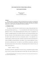
Fig. 1. Example dataset and skyline.
1. INTRODUCTION
The skyline operator is important for several applications involving multicrite-
ria decision making. Given a set of objects p
1
, p
2
, , p
N
, the operator returns
all objects p
i
such that p
i

is not dominated by another object p
j
. Using the
common example in the literature, assume in Figure 1 that we have a set of
hotels and for each hotel we store its distance from the beach (x axis) and its
price ( y axis). The most interesting hotels are a, i, and k, for which there is no
point that is better in both dimensions. Borzsonyi et al. [2001] proposed an SQL
syntax for the skyline operator, according to which the above query would be
expressed as: [Select *, From Hotels, Skyline of Price min, Distance min], where
min indicates that the price and the distance attributes should be minimized.
The syntax can also capture different conditions (such as max), joins, group-by,
and so on.
For simplicity, we assume that skylines are computed with respect to min con-
ditions on all dimensions; however, all methods discussed can be applied with
any combination of conditions. Using the min condition, a point p
i
dominates
1
another point p
j
if and only if the coordinate of p
i
on any axis is not larger than
the corresponding coordinate of p
j
. Informally, this implies that p
i
is preferable
to p
j

according to any preference (scoring) function which is monotone on all
attributes. For instance, hotel a in Figure 1 is better than hotels b and e since it
is closer to the beach and cheaper (independently of the relative importance of
the distance and price attributes). Furthermore, for every point p in the skyline
there exists a monotone function f such that p minimizes f [Borzsonyi et al.
2001].
Skylines are related to several other well-known problems, including convex
hulls, top-K queries, and nearest-neighbor search. In particular, the convex hull
contains the subset of skyline points that may be optimal only for linear pref-
erence functions (as opposed to any monotone function). B
¨
ohm and Kriegel
[2001] proposed an algorithm for convex hulls, which applies branch-and-
bound search on datasets indexed by R-trees. In addition, several main-memory
1
According to this definition, two or more points with the same coordinates can be part of the
skyline.
ACM Transactions on Database Systems, Vol. 30, No. 1, March 2005.
Progressive Skyline Computation in Database Systems
•
43
algorithms have been proposed for the case that the whole dataset fits in mem-
ory [Preparata and Shamos 1985].
Top-K (or ranked) queries retrieve the best K objects that minimize a specific
preference function. As an example, given the preference function f (x, y) =
x + y, the top-3 query, for the dataset in Figure 1, retrieves < i,5>, < h,7>,
< m,8> (in this order), where the number with each point indicates its score.
The difference from skyline queries is that the output changes according to the
input function and the retrieved points are not guaranteed to be part of the
skyline (h and m are dominated by i). Database techniques for top-K queries

include Prefer [Hristidis et al. 2001] and Onion [Chang et al. 2000], which are
based on prematerialization and convex hulls, respectively. Several methods
have been proposed for combining the results of multiple top-K queries [Fagin
et al. 2001; Natsev et al. 2001].
Nearest-neighbor queries specify a query point q and output the objects clos-
est to q,inincreasing order of their distance. Existing database algorithms as-
sume that the objects are indexed by an R-tree (or some other data-partitioning
method) and apply branch-and-bound search. In particular, the depth-first al-
gorithm of Roussopoulos et al. [1995] starts from the root of the R-tree and re-
cursively visits the entry closest to the query point. Entries, which are farther
than the nearest neighbor already found, are pruned. The best-first algorithm
of Henrich [1994] and Hjaltason and Samet [1999] inserts the entries of the
visited nodes in a heap, and follows the one closest to the query point. The re-
lation between skyline queries and nearest-neighbor search has been exploited
by previous skyline algorithms and will be discussed in Section 2.
Skylines, and other directly related problems such as multiobjective opti-
mization [Steuer 1986], maximum vectors [Kung et al. 1975; Matousek 1991],
and the contour problem [McLain 1974], have been extensively studied and nu-
merous algorithms have been proposed for main-memory processing. To the best
of our knowledge, however, the first work addressing skylines in the context of
databases was Borzsonyi et al. [2001], which develops algorithms based on block
nested loops, divide-and-conquer, and index scanning. An improved version of
block nested loops is presented in Chomicki et al. [2003]. Tan et al. [2001] pro-
posed progressive (or on-line) algorithms that can output skyline points without
having to scan the entire data input. Kossmann et al. [2002] presented an algo-
rithm, called NN due to its reliance on nearest-neighbor search, which applies
the divide-and-conquer framework on datasets indexed by R-trees. The exper-
imental evaluation of Kossmann et al. [2002] showed that NN outperforms
previous algorithms in terms of overall performance and general applicability
independently of the dataset characteristics, while it supports on-line process-

ing efficiently.
Despite its advantages, NN has also some serious shortcomings such as
need for duplicate elimination, multiple node visits, and large space require-
ments. Motivated by this fact, we propose a progressive algorithm called branch
and bound skyline (BBS), which, like NN, is based on nearest-neighbor search
on multidimensional access methods, but (unlike NN) is optimal in terms of
node accesses. We experimentally and analytically show that BBS outper-
forms NN (usually by orders of magnitude) for all problem instances, while
ACM Transactions on Database Systems, Vol. 30, No. 1, March 2005.
44
•
D. Papadias et al.
Fig. 2. Divide-and-conquer.
incurring less space overhead. In addition to its efficiency, the proposed algo-
rithm is simple and easily extendible to several practical variations of skyline
queries.
The rest of the article is organized as follows: Section 2 reviews previous
secondary-memory algorithms for skyline computation, discussing their advan-
tages and limitations. Section 3 introduces BBS, proves its optimality, and an-
alyzes its performance and space consumption. Section 4 proposes alternative
skyline queries and illustrates their processing using BBS. Section 5 introduces
the concept of approximate skylines, and Section 6 experimentally evaluates
BBS, comparing it against NN under a variety of settings. Finally, Section 7
concludes the article and describes directions for future work.
2. RELATED WORK
This section surveys existing secondary-memory algorithms for computing sky-
lines, namely: (1) divide-and-conquer, (2) block nested loop, (3) sort first skyline,
(4) bitmap, (5) index, and (6) nearest neighbor. Specifically, (1) and (2) were pro-
posed in Borzsonyi et al. [2001], (3) in Chomicki et al. [2003], (4) and (5) in Tan
et al. [2001], and (6) in Kossmann et al. [2002]. We do not consider the sorted list

scan, and the B-tree algorithms of Borzsonyi et al. [2001] due to their limited
applicability (only for two dimensions) and poor performance, respectively.
2.1 Divide-and-Conquer
The divide-and-conquer (D&C) approach divides the dataset into several par-
titions so that each partition fits in memory. Then, the partial skyline of the
points in every partition is computed using a main-memory algorithm (e.g.,
Matousek [1991]), and the final skyline is obtained by merging the partial ones.
Figure 2 shows an example using the dataset of Figure 1. The data space is di-
vided into four partitions s
1
, s
2
, s
3
, s
4
, with partial skylines {a, c, g}, {d}, {i},
{m, k}, respectively. In order to obtain the final skyline, we need to remove
those points that are dominated by some point in other partitions. Obviously
all points in the skyline of s
3
must appear in the final skyline, while those in s
2
ACM Transactions on Database Systems, Vol. 30, No. 1, March 2005.
Progressive Skyline Computation in Database Systems
•
45
are discarded immediately because they are dominated by any point in s
3
(in

fact s
2
needs to be considered only if s
3
is empty). Each skyline point in s
1
is
compared only with points in s
3
, because no point in s
2
or s
4
can dominate those
in s
1
.Inthis example, points c, g are removed because they are dominated by
i. Similarly, the skyline of s
4
is also compared with points in s
3
, which results in
the removal of m.Finally, the algorithm terminates with the remaining points
{a, i, k}. D&C is efficient only for small datasets (e.g., if the entire dataset fits
in memory then the algorithm requires only one application of a main-memory
skyline algorithm). For large datasets, the partitioning process requires read-
ing and writing the entire dataset at least once, thus incurring significant I/O
cost. Further, this approach is not suitable for on-line processing because it
cannot report any skyline until the partitioning phase completes.
2.2 Block Nested Loop and Sort First Skyline

A straightforward approach to compute the skyline is to compare each point p
with every other point, and report p as part of the skyline if it is not dominated.
Block nested loop (BNL) builds on this concept by scanning the data file and
keeping a list of candidate skyline points in main memory. At the beginning,
the list contains the first data point, while for each subsequent point p, there
are three cases: (i) if p is dominated by any point in the list, it is discarded as it
is not part of the skyline; (ii) if p dominates any point in the list, it is inserted,
and all points in the list dominated by p are dropped; and (iii) if p is neither
dominated by, nor dominates, any point in the list, it is simply inserted without
dropping any point.
The list is self-organizing because every point found dominating other points
is moved to the top. This reduces the number of comparisons as points that
dominate multiple other points are likely to be checked first. A problem of BNL
is that the list may become larger than the main memory. When this happens,
all points falling in the third case (cases (i) and (ii) do not increase the list size)
are added to a temporary file. This fact necessitates multiple passes of BNL. In
particular, after the algorithm finishes scanning the data file, only points that
were inserted in the list before the creation of the temporary file are guaranteed
to be in the skyline and are output. The remaining points must be compared
against the ones in the temporary file. Thus, BNL has to be executed again,
this time using the temporary (instead of the data) file as input.
The advantage of BNL is its wide applicability, since it can be used for any
dimensionality without indexing or sorting the data file. Its main problems are
the reliance on main memory (a small memory may lead to numerous iterations)
and its inadequacy for progressive processing (it has to read the entire data file
before it returns the first skyline point). The sort first skyline (SFS) variation
of BNL alleviates these problems by first sorting the entire dataset according
to a (monotone) preference function. Candidate points are inserted into the list
in ascending order of their scores, because points with lower scores are likely to
dominate a large number of points, thus rendering the pruning more effective.

SFS exhibits progressive behavior because the presorting ensures that a point
p dominating another p

must be visited before p

; hence we can immediately
ACM Transactions on Database Systems, Vol. 30, No. 1, March 2005.
46
•
D. Papadias et al.
Table I. The Bitmap Approach
id Coordinate Bitmap Representation
a (1, 9) (1111111111, 1100000000)
b (2, 10) (1111111110, 1000000000)
c (4, 8) (1111111000, 1110000000)
d (6, 7) (1111100000, 1111000000)
e (9, 10) (1100000000, 1000000000)
f (7, 5) (1111000000, 1111110000)
g (5, 6) (1111110000, 1111100000)
h (4, 3) (1111111000, 1111111100)
i (3, 2) (1111111100, 1111111110)
k (9, 1) (1100000000, 1111111111)
l (10, 4) (1000000000, 1111111000)
m (6, 2) (1111100000, 11111111110)
n (8, 3) (1110000000, 1111111100)
output the points inserted to the list as skyline points. Nevertheless, SFS has
to scan the entire data file to return a complete skyline, because even a skyline
point may have a very large score and thus appear at the end of the sorted list
(e.g., in Figure 1, point a has the third largest score for the preference function
0 · distance + 1 · price). Another problem of SFS (and BNL) is that the order in

which the skyline points are reported is fixed (and decided by the sort order),
while as discussed in Section 2.6, a progressive skyline algorithm should be
able to report points according to user-specified scoring functions.
2.3 Bitmap
This technique encodes in bitmaps all the information needed to decide whether
a point is in the skyline. Toward this, a data point p = (p
1
, p
2
, , p
d
), where
d is the number of dimensions, is mapped to an m-bit vector, where m is the
total number of distinct values over all dimensions. Let k
i
be the total number
of distinct values on the ith dimension (i.e., m =

i=1∼d
k
i
). In Figure 1, for
example, there are k
1
= k
2
= 10 distinct values on the x, y dimensions and
m = 20. Assume that p
i
is the j

i
th smallest number on the ith axis; then it
is represented by k
i
bits, where the leftmost (k
i
− j
i
+ 1) bits are 1, and the
remaining ones 0. Table I shows the bitmaps for points in Figure 1. Since point
a has the smallest value (1) on the x axis, all bits of a
1
are 1. Similarly, since
a
2
(= 9) is the ninth smallest on the y axis, the first 10 − 9 + 1 = 2 bits of its
representation are 1, while the remaining ones are 0.
Consider that we want to decide whether a point, for example, c with bitmap
representation (1111111000, 1110000000), belongs to the skyline. The right-
most bits equal to 1, are the fourth and the eighth, on dimensions x and y,
respectively. The algorithm creates two bit-strings, c
X
= 1110000110000 and
c
Y
= 0011011111111, by juxtaposing the corresponding bits (i.e., the fourth
and eighth) of every point. In Table I, these bit-strings (shown in bold) contain
13 bits (one from each object, starting from a and ending with n). The 1s in the
result of c
X

& c
Y
= 0010000110000 indicate the points that dominate c, that
is, c, h, and i. Obviously, if there is more than a single 1, the considered point
ACM Transactions on Database Systems, Vol. 30, No. 1, March 2005.
Progressive Skyline Computation in Database Systems
•
47
Table II. The Index Approach
List 1 List 2
a (1, 9) minC = 1 k (9, 1) minC = 1
b (2, 10) minC = 2 i (3, 2), m (6, 2) minC = 2
c (4, 8) minC = 4 h (4, 3), n (8, 3) minC = 3
g (5, 6) minC = 5 l (10, 4) minC = 4
d (6, 7) minC = 6 f (7, 5) minC = 5
e (9, 10) minC = 9
is not in the skyline.
2
The same operations are repeated for every point in the
dataset to obtain the entire skyline.
The efficiency of bitmap relies on the speed of bit-wise operations. The ap-
proach can quickly return the first few skyline points according to their inser-
tion order (e.g., alphabetical order in Table I), but, as with BNL and SFS, it
cannot adapt to different user preferences. Furthermore, the computation of
the entire skyline is expensive because, for each point inspected, it must re-
trieve the bitmaps of all points in order to obtain the juxtapositions. Also the
space consumption may be prohibitive, if the number of distinct values is large.
Finally, the technique is not suitable for dynamic datasets where insertions
may alter the rankings of attribute values.
2.4 Index

The index approach organizes a set of d -dimensional points into d lists such
that a point p = ( p
1
, p
2
, , p
d
)isassigned to the ith list (1 ≤ i ≤ d ), if and
only if its coordinate p
i
on the ith axis is the minimum among all dimensions, or
formally, p
i
≤ p
j
for all j = i.Table II shows the lists for the dataset of Figure 1.
Points in each list are sorted in ascending order of their minimum coordinate
(minC, for short) and indexed by a B-tree. A batch in the ith list consists of
points that have the same ith coordinate (i.e., minC). In Table II, every point
of list 1 constitutes an individual batch because all x coordinates are different.
Points in list 2 are divided into five batches {k}, {i, m}, {h, n}, {l}, and { f }.
Initially, the algorithm loads the first batch of each list, and handles the one
with the minimum minC.InTable II, the first batches {a}, {k} have identical
minC = 1, in which case the algorithm handles the batch from list 1. Processing
a batch involves (i) computing the skyline inside the batch, and (ii) among the
computed points, it adds the ones not dominated by any of the already-found
skyline points into the skyline list. Continuing the example, since batch {a}
contains a single point and no skyline point is found so far, a is added to the
skyline list. The next batch {b} in list 1 has minC = 2; thus, the algorithm
handles batch {k} from list 2. Since k is not dominated by a,itisinserted in

the skyline. Similarly, the next batch handled is {b} from list 1, where b is
dominated by point a (already in the skyline). The algorithm proceeds with
batch {i, m}, computes the skyline inside the batch that contains a single point
i (i.e., i dominates m), and adds i to the skyline. At this step, the algorithm does
2
The result of “&” will contain several 1s if multiple skyline points coincide. This case can be
handled with an additional “or” operation [Tan et al. 2001].
ACM Transactions on Database Systems, Vol. 30, No. 1, March 2005.
48
•
D. Papadias et al.
Fig. 3. Example of NN.
not need to proceed further, because both coordinates of i are smaller than or
equal to the minC (i.e., 4, 3) of the next batches (i.e., {c}, {h, n})oflists 1 and
2. This means that all the remaining points (in both lists) are dominated by i,
and the algorithm terminates with {a, i, k}.
Although this technique can quickly return skyline points at the top of the
lists, the order in which the skyline points are returned is fixed, not supporting
user-defined preferences. Furthermore, as indicated in Kossmann et al. [2002],
the lists computed for d dimensions cannot be used to retrieve the skyline on any
subset of the dimensions because the list that an element belongs to may change
according the subset of selected dimensions. In general, for supporting queries
on arbitrary dimensions, an exponential number of lists must be precomputed.
2.5 Nearest Neighbor
NN uses the results of nearest-neighbor search to partition the data universe
recursively. As an example, consider the application of the algorithm to the
dataset of Figure 1, which is indexed by an R-tree [Guttman 1984; Sellis et al.
1987; Beckmann et al. 1990]. NN performs a nearest-neighbor query (using an
existing algorithm such as one of the proposed by Roussopoulos et al. [1995], or
Hjaltason and Samet [1999] on the R-tree, to find the point with the minimum

distance (mindist) from the beginning of the axes (point o). Without loss of
generality,
3
we assume that distances are computed according to the L
1
norm,
that is, the mindist of a point p from the beginning of the axes equals the sum
of the coordinates of p.Itcan be shown that the first nearest neighbor (point
i with mindist 5) is part of the skyline. On the other hand, all the points in
the dominance region of i (shaded area in Figure 3(a)) can be pruned from
further consideration. The remaining space is split in two partitions based on
the coordinates (i
x
, i
y
)ofpoint i: (i) [0, i
x
) [0, ∞) and (ii) [0, ∞) [0, i
y
). In
Figure 3(a), the first partition contains subdivisions 1 and 3, while the second
one contains subdivisions 1 and 2.
The partitions resulting after the discovery of a skyline point are inserted in
a to-do list. While the to-do list is not empty, NN removes one of the partitions
3
NN (and BBS) can be applied with any monotone function; the skyline points are the same, but
the order in which they are discovered may be different.
ACM Transactions on Database Systems, Vol. 30, No. 1, March 2005.
Progressive Skyline Computation in Database Systems
•

49
Fig. 4. NN partitioning for three-dimensions.
from the list and recursively repeats the same process. For instance, point a is
the nearest neighbor in partition [0, i
x
) [0, ∞), which causes the insertion of
partitions [0, a
x
) [0, ∞) (subdivisions 5 and 7 in Figure 3(b)) and [0, i
x
) [0, a
y
)
(subdivisions 5 and 6 in Figure 3(b)) in the to-do list. If a partition is empty, it is
not subdivided further. In general, if d is the dimensionality of the data-space,
a new skyline point causes d recursive applications of NN. In particular, each
coordinate of the discovered point splits the corresponding axis, introducing a
new search region towards the origin of the axis.
Figure 4(a) shows a three-dimensional (3D) example, where point n with
coordinates (n
x
, n
y
, n
z
)isthe first nearest neighbor (i.e., skyline point). The NN
algorithm will be recursively called for the partitions (i) [0, n
x
) [0, ∞) [0, ∞)
(Figure 4(b)), (ii) [0, ∞) [0, n

y
) [0, ∞)(Figure 4(c)) and (iii) [0, ∞) [0, ∞) [0, n
z
)
(Figure 4(d)). Among the eight space subdivisions shown in Figure 4, the eighth
one will not be searched by any query since it is dominated by point n. Each
of the remaining subdivisions, however, will be searched by two queries, for
example, a skyline point in subdivision 2 will be discovered by both the second
and third queries.
In general, for d > 2, the overlapping of the partitions necessitates dupli-
cate elimination. Kossmann et al. [2002] proposed the following elimination
methods:
—Laisser-faire: A main memory hash table stores the skyline points found so
far. When a point p is discovered, it is probed and, if it already exists in the
hash table, p is discarded; otherwise, p is inserted into the hash table. The
technique is straightforward and incurs minimum CPU overhead, but results
in very high I/O cost since large parts of the space will be accessed by multiple
queries.
—Propagate: When a point p is found, all the partitions in the to-do list that
contain p are removed and repartitioned according to p. The new partitions
are inserted into the to-do list. Although propagate does not discover the same
ACM Transactions on Database Systems, Vol. 30, No. 1, March 2005.
50
•
D. Papadias et al.
skyline point twice, it incurs high CPU cost because the to-do list is scanned
every time a skyline point is discovered.
—Merge: The main idea is to merge partitions in to-do, thus reducing the num-
ber of queries that have to be performed. Partitions that are contained in
other ones can be eliminated in the process. Like propagate, merge also in-

curs high CPU cost since it is expensive to find good candidates for merging.
—Fine-grained partitioning: The original NN algorithm generates d partitions
after a skyline point is found. An alternative approach is to generate 2
d
nonoverlapping subdivisions. In Figure 4, for instance, the discovery of point
n will lead to six new queries (i.e., 2
3
–2since subdivisions 1 and 8 cannot
contain any skyline points). Although fine-grained partitioning avoids dupli-
cates, it generates the more complex problem of false hits, that is, it is possible
that points in one subdivision (e.g., subdivision 4) are dominated by points
in another (e.g., subdivision 2) and should be eliminated.
According to the experimental evaluation of Kossmann et al. [2002], the
performance of laisser-faire and merge was unacceptable, while fine-grained
partitioning was not implemented due to the false hits problem. Propagate
was significantly more efficient, but the best results were achieved by a hybrid
method combining propagate and laisser-faire.
2.6 Discussion About the Existing Algorithms
We summarize this section with a comparison of the existing methods, based
on the experiments of Tan et al. [2001], Kossmann et al. [2002], and Chomicki
et al. [2003]. Tan et al. [2001] examined BNL, D&C, bitmap, and index, and
suggested that index is the fastest algorithm for producing the entire skyline
under all settings. D&C and bitmap are not favored by correlated datasets
(where the skyline is small) as the overhead of partition-merging and bitmap-
loading, respectively, does not pay-off. BNL performs well for small skylines,
but its cost increases fast with the skyline size (e.g., for anticorrelated datasets,
high dimensionality, etc.) due to the large number of iterations that must be
performed. Tan et al. [2001] also showed that index has the best performance in
returning skyline points progressively, followed by bitmap. The experiments of
Chomicki et al. [2003] demonstrated that SFS is in most cases faster than BNL

without, however, comparing it with other algorithms. According to the eval-
uation of Kossmann et al. [2002], NN returns the entire skyline more quickly
than index (hence also more quickly than BNL, D&C, and bitmap) for up to four
dimensions, and their difference increases (sometimes to orders of magnitudes)
with the skyline size. Although index can produce the first few skyline points in
shorter time, these points are not representative of the whole skyline (as they
are good on only one axis while having large coordinates on the others).
Kossmann et al. [2002] also suggested a set of criteria (adopted from Heller-
stein et al. [1999]) for evaluating the behavior and applicability of progressive
skyline algorithms:
(i) Progressiveness: the first results should be reported to the user almost
instantly and the output size should gradually increase.
ACM Transactions on Database Systems, Vol. 30, No. 1, March 2005.
Progressive Skyline Computation in Database Systems
•
51
(ii) Absence of false misses: given enough time, the algorithm should generate
the entire skyline.
(iii) Absence of false hits: the algorithm should not discover temporary skyline
points that will be later replaced.
(iv) Fairness: the algorithm should not favor points that are particularly good
in one dimension.
(v) Incorporation of preferences: the users should be able to determine the
order according to which skyline points are reported.
(vi) Universality: the algorithm should be applicable to any dataset distribu-
tion and dimensionality, using some standard index structure.
All the methods satisfy criterion (ii), as they deal with exact (as opposed to
approximate) skyline computation. Criteria (i) and (iii) are violated by D&C and
BNL since they require at least a scan of the data file before reporting skyline
points and they both insert points (in partial skylines or the self-organizing

list) that are later removed. Furthermore, SFS and bitmap need to read the
entire file before termination, while index and NN can terminate as soon as all
skyline points are discovered. Criteria (iv) and (vi) are violated by index because
it outputs the points according to their minimum coordinates in some dimension
and cannot handle skylines in some subset of the original dimensionality. All
algorithms, except NN, defy criterion (v); NN can incorporate preferences by
simply changing the distance definition according to the input scoring function.
Finally, note that progressive behavior requires some form of preprocessing,
that is, index creation (index, NN), sorting (SFS), or bitmap creation (bitmap).
This preprocessing is a one-time effort since it can be used by all subsequent
queries provided that the corresponding structure is updateable in the presence
of record insertions and deletions. The maintenance of the sorted list in SFS can
be performed by building a B+-tree on top of the list. The insertion of a record
in index simply adds the record in the list that corresponds to its minimum
coordinate; similarly, deletion removes the record from the list. NN can also
be updated incrementally as it is based on a fully dynamic structure (i.e., the
R-tree). On the other hand, bitmap is aimed at static datasets because a record
insertion/deletion may alter the bitmap representation of numerous (in the
worst case, of all) records.
3. BRANCH-AND-BOUND SKYLINE ALGORITHM
Despite its general applicability and performance advantages compared to ex-
isting skyline algorithms, NN has some serious shortcomings, which are de-
scribed in Section 3.1. Then Section 3.2 proposes the BBS algorithm and proves
its correctness. Section 3.3 analyzes the performance of BBS and illustrates its
I/O optimality. Finally, Section 3.4 discusses the incremental maintenance of
skylines in the presence of database updates.
3.1 Motivation
A recursive call of the NN algorithm terminates when the corresponding
nearest-neighbor query does not retrieve any point within the corresponding
ACM Transactions on Database Systems, Vol. 30, No. 1, March 2005.

52
•
D. Papadias et al.
Fig. 5. Recursion tree.
space. Lets call such a query empty,todistinguish it from nonempty queries
that return results, each spawning d new recursive applications of the algo-
rithm (where d is the dimensionality of the data space). Figure 5 shows a
query processing tree, where empty queries are illustrated as transparent cy-
cles. For the second level of recursion, for instance, the second query does not
return any results, in which case the recursion will not proceed further. Some
of the nonempty queries may be redundant, meaning that they return sky-
line points already found by previous queries. Let s be the number of skyline
points in the result, e the number of empty queries, ne the number of nonempty
ones, and r the number of redundant queries. Since every nonempty query
either retrieves a skyline point, or is redundant, we have ne = s + r. Fur-
thermore, the number of empty queries in Figure 5 equals the number of leaf
nodes in the recursion tree, that is, e = ne · (d − 1) + 1. By combining the two
equations, we get e = (s + r) · (d − 1) + 1. Each query must traverse a whole
path from the root to the leaf level of the R-tree before it terminates; there-
fore, its I/O cost is at least h node accesses, where h is the height of the tree.
Summarizing the above observations, the total number of accesses for NN is:
NA
NN
≥ (e + s + r) · h = (s + r) · h · d + h > s · h · d. The value s · h · d is a rather
optimistic lower bound since, for d > 2, the number r of redundant queries
may be very high (depending on the duplicate elimination method used), and
queries normally incur more than h node accesses.
Another problem of NN concerns the to-do list size, which can exceed that of
the dataset for as low as three dimensions, even without considering redundant
queries. Assume, for instance, a 3D uniform dataset (cardinality N) and a sky-

line query with the preference function f (x, y, z) = x. The first skyline point
n (n
x
, n
y
, n
z
) has the smallest x coordinate among all data points, and adds
partitions P
x
= [0, n
x
) [0, ∞) [0, ∞), P
y
= [0, ∞) [0, n
y
) [0, ∞), P
z
= [0, ∞)
[0, ∞) [0, n
z
)inthe to-do list. Note that the NN query in P
x
is empty because
there is no other point whose x coordinate is below n
x
.Onthe other hand, the
expected volume of P
y
(P

z
)is
1
/
2
(assuming unit axis length on all dimensions),
because the nearest neighbor is decided solely on x coordinates, and hence n
y
(n
z
) distributes uniformly in [0, 1]. Following the same reasoning, a NN in P
y
finds the second skyline point that introduces three new partitions such that
one partition leads to an empty query, while the volumes of the other two are
1
/
4
. P
z
is handled similarly, after which the to-do list contains four partitions
with volumes
1
/
4
, and 2 empty partitions. In general, after the ith level of re-
cursion, the to-do list contains 2
i
partitions with volume 1/2
i
, and 2

i−1
empty
ACM Transactions on Database Systems, Vol. 30, No. 1, March 2005.
Progressive Skyline Computation in Database Systems
•
53
Fig. 6. R-tree example.
partitions. The algorithm terminates when 1/2
i
< 1/N (i.e., i > log N)sothat
all partitions in the to-do list are empty. Assuming that the empty queries are
performed at the end, the size of the to-do list can be obtained by summing the
number e of empty queries at each recursion level i:
log N

i=1
2
i−1
= N − 1.
The implication of the above equation is that, even in 3D, NN may behave
like a main-memory algorithm (since the to-do list, which resides in memory,
is the same order of size as the input dataset). Using the same reasoning, for
arbitrary dimensionality d > 2, e = ((d −1)
log N
), that is, the to-do list may
become orders of magnitude larger than the dataset, which seriously limits
the applicability of NN. In fact, as shown in Section 6, the algorithm does not
terminate in the majority of experiments involving four and five dimensions.
3.2 Description of BBS
Like NN, BBS is also based on nearest-neighbor search. Although both algo-

rithms can be used with any data-partitioning method, in this article we use
R-trees due to their simplicity and popularity. The same concepts can be ap-
plied with other multidimensional access methods for high-dimensional spaces,
where the performance of R-trees is known to deteriorate. Furthermore, as
claimed in Kossmann et al. [2002], most applications involve up to five di-
mensions, for which R-trees are still efficient. For the following discussion, we
use the set of 2D data points of Figure 1, organized in the R-tree of Figure 6
with node capacity = 3. An intermediate entry e
i
corresponds to the minimum
bounding rectangle (MBR) of a node N
i
at the lower level, while a leaf entry
corresponds to a data point. Distances are computed according to L
1
norm, that
is, the mindist of a point equals the sum of its coordinates and the mindist of a
MBR (i.e., intermediate entry) equals the mindist of its lower-left corner point.
BBS, similar to the previous algorithms for nearest neighbors [Roussopoulos
et al. 1995; Hjaltason and Samet 1999] and convex hulls [B
¨
ohm and Kriegel
2001], adopts the branch-and-bound paradigm. Specifically, it starts from the
root node of the R-tree and inserts all its entries (e
6
, e
7
)inaheap sorted ac-
cording to their mindist. Then, the entry with the minimum mindist (e
7

)is
“expanded”. This expansion removes the entry (e
7
) from the heap and inserts
ACM Transactions on Database Systems, Vol. 30, No. 1, March 2005.
54
•
D. Papadias et al.
Table III. Heap Contents
Action Heap Contents S
Access root <e
7,
4><e
6,
6> Ø
Expand e
7
<e
3,
5><e
6,
6><e
5,
8><e
4,
10> Ø
Expand e
3
<i,5><e
6,

6><h, 7><e
5,
8> <e
4,
10><g, 11> {i}
Expand e
6
<h, 7><e
5
, 8><e
1,
9><e
4,
10><g, 11> {i}
Expand e
1
<a,10><e
4,
10><g, 11><b, 12><c, 12> {i, a}
Expand e
4
<k,10><g, 11>< b, 12>< c, 12>< l, 14> {i, a, k}
Fig. 7. BBS algorithm.
its children (e
3
, e
4
, e
5
). The next expanded entry is again the one with the min-

imum mindist (e
3
), in which the first nearest neighbor (i)isfound. This point
(i) belongs to the skyline, and is inserted to the list S of skyline points.
Notice that up to this step BBS behaves like the best-first nearest-neighbor
algorithm of Hjaltason and Samet [1999]. The next entry to be expanded is
e
6
. Although the nearest-neighbor algorithm would now terminate since the
mindist (6) of e
6
is greater than the distance (5) of the nearest neighbor (i)
already found, BBS will proceed because node N
6
may contain skyline points
(e.g., a). Among the children of e
6
, however, only the ones that are not dominated
by some point in S are inserted into the heap. In this case, e
2
is pruned because
it is dominated by point i. The next entry considered (h)isalso pruned as it
also is dominated by point i. The algorithm proceeds in the same manner until
the heap becomes empty. Table III shows the ids and the mindist of the entries
inserted in the heap (skyline points are bold).
The pseudocode for BBS is shown in Figure 7. Notice that an entry is checked
for dominance twice: before it is inserted in the heap and before it is expanded.
The second check is necessary because an entry (e.g., e
5
)inthe heap may become

dominated by some skyline point discovered after its insertion (therefore, the
entry does not need to be visited).
Next we prove the correctness for BBS.
L
EMMA 1. BBS visits (leaf and intermediate) entries of an R-tree in ascend-
ing order of their distance to the origin of the axis.
ACM Transactions on Database Systems, Vol. 30, No. 1, March 2005.
Progressive Skyline Computation in Database Systems
•
55
Fig. 8. Entries of the main-memory R-tree.
PROOF. The proof is straightforward since the algorithm always visits en-
tries according to their mindist order preserved by the heap.
LEMMA 2. Any data point added to S during the execution of the algorithm
is guaranteed to be a final skyline point.
P
ROOF. Assume, on the contrary, that point p
j
was added into S, but it is not
a final skyline point. Then p
j
must be dominated by a (final) skyline point, say,
p
i
, whose coordinate on any axis is not larger than the corresponding coordinate
of p
j
, and at least one coordinate is smaller (since p
i
and p

j
are different points).
This in turn means that mindist(p
i
) < mindist( p
j
). By Lemma 1, p
i
must be
visited before p
j
.Inother words, at the time p
j
is processed, p
i
must have
already appeared in the skyline list, and hence p
j
should be pruned, which
contradicts the fact that p
j
was added in the list.
LEMMA 3. Every data point will be examined, unless one of its ancestor nodes
has been pruned.
P
ROOF. The proof is obvious since all entries that are not pruned by an
existing skyline point are inserted into the heap and examined.
Lemmas 2 and 3 guarantee that, if BBS is allowed to execute until its ter-
mination, it will correctly return all skyline points, without reporting any false
hits. An important issue regards the dominance checking, which can be expen-

sive if the skyline contains numerous points. In order to speed up this process
we insert the skyline points found in a main-memory R-tree. Continuing the
example of Figure 6, for instance, only points i, a, k will be inserted (in this
order) to the main-memory R-tree. Checking for dominance can now be per-
formed in a way similar to traditional window queries. An entry (i.e., node
MBR or data point) is dominated by a skyline point p,ifits lower left point
falls inside the dominance region of p, that is, the rectangle defined by p and
the edge of the universe. Figure 8 shows the dominance regions for points i,
a, k and two entries; e is dominated by i and k, while e

is not dominated by
any point (therefore is should be expanded). Note that, in general, most domi-
nance regions will cover a large part of the data space, in which case there will
be significant overlap between the intermediate nodes of the main-memory
ACM Transactions on Database Systems, Vol. 30, No. 1, March 2005.
56
•
D. Papadias et al.
R-tree. Unlike traditional window queries that must retrieve all results, this
is not a problem here because we only need to retrieve a single dominance re-
gion in order to determine that the entry is dominated (by at least one skyline
point).
To conclude this section, we informally evaluate BBS with respect to the
criteria of Hellerstein et al. [1999] and Kossmann et al. [2002], presented in
Section 2.6. BBS satisfies property (i) as it returns skyline points instantly in
ascending order of their distance to the origin, without having to visit a large
part of the R-tree. Lemma 3 ensures property (ii), since every data point is
examined unless some of its ancestors is dominated (in which case the point is
dominated too). Lemma 2 guarantees property (iii). Property (iv) is also fulfilled
because BBS outputs points according to their mindist, which takes into account

all dimensions. Regarding user preferences (v), as we discuss in Section 4.1,
the user can specify the order of skyline points to be returned by appropriate
preference functions. Furthermore, BBS also satisfies property (vi) since it does
not require any specialized indexing structure, but (like NN) it can be applied
with R-trees or any other data-partitioning method. Furthermore, the same
index can be used for any subset of the d dimensions that may be relevant to
different users.
3.3 Analysis of BBS
In this section, we first prove that BBS is I/O optimal, meaning that (i) it visits
only the nodes that may contain skyline points, and (ii) it does not access the
same node twice. Then we provide a theoretical comparison with NN in terms
of the number of node accesses and memory consumption (i.e., the heap versus
the to-do list sizes). Central to the analysis of BBS is the concept of the skyline
search region (SSR), that is, the part of the data space that is not dominated
by any skyline point. Consider for instance the running example (with skyline
points i, a, k). The SSR is the shaded area in Figure 8 defined by the skyline
and the two axes. We start with the following observation.
L
EMMA 4. Any skyline algorithm based on R-trees must access all the nodes
whose MBRs intersect the SSR.
For instance, although entry e

in Figure 8 does not contain any skyline points,
this cannot be determined unless the child node of e

is visited.
L
EMMA 5. If an entry e does not intersect the SSR, then there is a skyline
point p whose distance from the origin of the axes is smaller than the mindist
of e.

P
ROOF. Since e does not intersect the SSR,itmust be dominated by at
least one skyline point p, meaning that p dominates the lower-left corner of
e. This implies that the distance of p to the origin is smaller than the mindist
of e.
THEOREM 6. The number of node accesses performed by BBS is optimal.
ACM Transactions on Database Systems, Vol. 30, No. 1, March 2005.
Progressive Skyline Computation in Database Systems
•
57
PROOF
.First we prove that BBS only accesses nodes that may contain sky-
line points. Assume, to the contrary, that the algorithm also visits an entry
(let it be e in Figure 8) that does not intersect the SSR. Clearly, e should not
be accessed because it cannot contain skyline points. Consider a skyline point
that dominates e (e.g., k). Then, by Lemma 5, the distance of k to the origin is
smaller than the mindist of e. According to Lemma 1, BBS visits the entries of
the R-tree in ascending order of their mindist to the origin. Hence, k must be
processed before e, meaning that e will be pruned by k, which contradicts the
fact that e is visited.
In order to complete the proof, we need to show that an entry is not visited
multiple times. This is straightforward because entries are inserted into the
heap (and expanded) at most once, according to their mindist.
Assuming that each leaf node visited contains exactly one skyline point, the
number NA
BBS
of node accesses performed by BBS is at most s · h (where s
is the number of skyline points, and h the height of the R-tree). This bound
corresponds to a rather pessimistic case, where BBS has to access a complete
path for each skyline point. Many skyline points, however, may be found in the

same leaf nodes, or in the same branch of a nonleaf node (e.g., the root of the
tree!), so that these nodes only need to be accessed once (our experiments show
that in most cases the number of node accesses at each level of the tree is much
smaller than s). Therefore, BBS is at least d (= s·h·d /s·h) times faster than NN
(as explained in Section 3.1, the cost NA
NN
of NN is at least s ·h· d ). In practice,
for d > 2, the speedup is much larger than d (several orders of magnitude) as
NA
NN
= s · h · d does not take into account the number r of redundant queries.
Regarding the memory overhead, the number of entries n
heap
in the heap of
BBS is at most ( f − 1) · NA
BBS
. This is a pessimistic upper bound, because it
assumes that a node expansion removes from the heap the expanded entry and
inserts all its f children (in practice, most children will be dominated by some
discovered skyline point and pruned). Since for independent dimensions the
expected number of skyline points is s = ((ln N )
d−1
/(d − 1)!) (Buchta [1989]),
n
heap
≤ ( f − 1) · NA
BBS
≈ ( f − 1) · h · s ≈ ( f − 1) · h · (ln N)
d−1
/(d − 1)!. For

d ≥ 3 and typical values of N and f (e.g., N = 10
5
and f ≈ 100), the heap
size is much smaller than the corresponding to-do list size, which as discussed
in Section 3.1 can be in the order of (d − 1)
log N
. Furthermore, a heap entry
stores d + 2 numbers (i.e., entry id, mindist, and the coordinates of the lower-
left corner), as opposed to 2d numbers for to-do list entries (i.e., d-dimensional
ranges).
In summary, the main-memory requirement of BBS is at the same order
as the size of the skyline, since both the heap and the main-memory R-tree
sizes are at this order. This is a reasonable assumption because (i) skylines
are normally small and (ii) previous algorithms, such as index, are based on
the same principle. Nevertheless, the size of the heap can be further reduced.
Consider that in Figure 9 intermediate node e is visited first and its children
(e.g., e
1
) are inserted into the heap. When e

is visited afterward (e and e

have
the same mindist), e

1
can be immediately pruned, because there must exist at
least a (not yet discovered) point in the bottom edge of e
1
that dominates e


1
.A
ACM Transactions on Database Systems, Vol. 30, No. 1, March 2005.
58
•
D. Papadias et al.
Fig. 9. Reducing the size of the heap.
similar situation happens if node e

is accessed first. In this case e

1
is inserted
into the heap, but it is removed (before its expansion) when e
1
is added. BBS
can easily incorporate this mechanism by checking the contents of the heap
before the insertion of an entry e: (i) all entries dominated by e are removed;
(ii) if e is dominated by some entry, it is not inserted. We chose not to implement
this optimization because it induces some CPU overhead without affecting the
number of node accesses, which is optimal (in the above example e

1
would be
pruned during its expansion since by that time e
1
will have been visited).
3.4 Incremental Maintenance of the Skyline
The skyline may change due to subsequent updates (i.e., insertions and dele-

tions) to the database, and hence should be incrementally maintained to avoid
recomputation. Given a new point p (e.g., a hotel added to the database), our
incremental maintenance algorithm first performs a dominance check on the
main-memory R-tree. If p is dominated (by an existing skyline point), it is sim-
ply discarded (i.e., it does not affect the skyline); otherwise, BBS performs a
window query (on the main-memory R-tree), using the dominance region of p,
to retrieve the skyline points that will become obsolete (i.e., those dominated by
p). This query may not retrieve anything (e.g., Figure 10(a)), in which case the
number of skyline points increases by one. Figure 10(b) shows another case,
where the dominance region of p covers two points i, k, which are removed
(from the main-memory R-tree). The final skyline consists of only points a, p.
Handling deletions is more complex. First, if the point removed is not in
the skyline (which can be easily checked by the main-memory R-tree using
the point’s coordinates), no further processing is necessary. Otherwise, part
of the skyline must be reconstructed. To illustrate this, assume that point i in
Figure 11(a) is deleted. For incremental maintenance, we need to compute the
skyline with respect only to the points in the constrained (shaded) area, which
is the region exclusively dominated by i (i.e., not including areas dominated by
other skyline points). This is because points (e.g., e, l) outside the shaded area
cannot appear in the new skyline, as they are dominated by at least one other
point (i.e., a or k). As shown in Figure 11(b), the skyline within the exclusive
dominance region of i contains two points h and m, which substitute i in the final
ACM Transactions on Database Systems, Vol. 30, No. 1, March 2005.
Progressive Skyline Computation in Database Systems
•
59
Fig. 10. Incremental skyline maintenance for insertion.
Fig. 11. Incremental skyline maintenance for deletion.
skyline (of the whole dataset). In Section 4.1, we discuss skyline computation
in a constrained region of the data space.

Except for the above case of deletion, incremental skyline maintenance in-
volves only main-memory operations. Given that the skyline points constitute
only a small fraction of the database, the probability of deleting a skyline point
is expected to be very low. In extreme cases (e.g., bulk updates, large num-
ber of skyline points) where insertions/deletions frequently affect the skyline,
we may adopt the following “lazy” strategy to minimize the number of disk
accesses: after deleting a skyline point p,wedonot compute the constrained
skyline immediately, but add p to a buffer. For each subsequent insertion, if p
is dominated by a new point p

,weremove it from the buffer because all the
points potentially replacing p would become obsolete anyway as they are dom-
inated by p

(the insertion of p

may also render other skyline points obsolete).
When there are no more updates or a user issues a skyline query, we perform
a single constrained skyline search, setting the constraint region to the union
of the exclusive dominance regions of the remaining points in the buffer, which
is emptied afterward.
ACM Transactions on Database Systems, Vol. 30, No. 1, March 2005.
60
•
D. Papadias et al.
Fig. 12. Constrained query example.
4. VARIATIONS OF SKYLINE QUERIES
In this section we propose novel variations of skyline search, and illustrate how
BBS can be applied for their processing. In particular, Section 4.1 discusses
constrained skylines, Section 4.2 ranked skylines, Section 4.3 group-by sky-

lines, Section 4.4 dynamic skylines, Section 4.5 enumerating and K -dominating
queries, and Section 4.6 skybands.
4.1 Constrained Skyline
Given a set of constraints, a constrained skyline query returns the most in-
teresting points in the data space defined by the constraints. Typically, each
constraint is expressed as a range along a dimension and the conjunction of all
constraints forms a hyperrectangle (referred to as the constraint region)inthe
d-dimensional attribute space. Consider the hotel example, where a user is in-
terested only in hotels whose prices ( y axis) are in the range [4, 7]. The skyline
in this case contains points g, f , and l (Figure 12), as they are the most inter-
esting hotels in the specified price range. Note that d (which also satisfies the
constraints) is not included as it is dominated by g. The constrained query can
be expressed using the syntax of Borzsonyi et al. [2001] and the where clause:
Select *, From Hotels, Where Price∈[4, 7], Skyline of Price min, Distance min.
In addition, constrained queries are useful for incremental maintenance of the
skyline in the presence of deletions (as discussed in Section 3.4).
BBS can easily process such queries. The only difference with respect to the
original algorithm is that entries not intersecting the constraint region are
pruned (i.e., not inserted in the heap). Table IV shows the contents of the heap
during the processing of the query in Figure 12. The same concept can also be
applied when the constraint region is not a (hyper-) rectangle, but an arbitrary
area in the data space.
The NN algorithm can also support constrained skylines with a similar
modification. In particular, the first nearest neighbor (e.g., g)isretrieved in
the constraint region using constrained nearest-neighbor search [Ferhatosman-
oglu et al. 2001]. Then, each space subdivision is the intersection of the origi-
nal subdivision (area to be searched by NN for the unconstrained query) and
the constraint region. The index method can benefit from the constraints, by
ACM Transactions on Database Systems, Vol. 30, No. 1, March 2005.
Progressive Skyline Computation in Database Systems

•
61
Table IV. Heap Contents for Constrained Query
Action Heap Contents S
Access root <e
7
, 4><e
6
,6> Ø
Expand e
7
<e
3
, 5><e
6
, 6><e
4
, 10> Ø
Expand e
3
<e
6
,6><e
4
, 10><g, 11> Ø
Expand e
6
<e
4
, 10><g, 11><e

2
, 11> Ø
Expand e
4
<g, 11><e
2
, 11><l, 14> {g}
Expand e
2
<f, 12><d, 13><l, 14> {g, f, l}
starting with the batches at the beginning of the constraint ranges (instead of
the top of the lists). Bitmap can avoid loading the juxtapositions (see Section
2.3) for points that do not satisfy the query constraints, and D&C may discard,
during the partitioning step, points that do not belong to the constraint region.
For BNL and SFS, the only difference with respect to regular skyline retrieval is
that only points in the constraint region are inserted in the self-organizing list.
4.2 Ranked Skyline
Given a set of points in the d -dimensional space [0, 1]
d
,aranked (top-K ) sky-
line query (i) specifies a parameter K , and a preference function f which is
monotone on each attribute, (ii) and returns the K skyline points p that have
the minimum score according to the input function. Consider the running exam-
ple, where K = 2 and the preference function is f (x, y) = x + 3 y
2
. The output
skyline points should be < k,12 >, < i,15 > in this order (the number with
each point indicates its score). Such ranked skyline queries can be expressed
using the syntax of Borzsonyi et al. [2001] combined with the order by and stop
after clauses: Select *, From Hotels, Skyline of Price min, Distance min, order

by Price + 3·sqr(Distance), stop after 2.
BBS can easily handle such queries by modifying the mindist definition to
reflect the preference function (i.e., the mindist of a point with coordinates x
and y equals x + 3 y
2
). The mindist of an intermediate entry equals the score
of its lower-left point. Furthermore, the algorithm terminates after exactly K
points have been reported. Due to the monotonicity of f ,itiseasy to prove that
the output points are indeed skyline points. The only change with respect to
the original algorithm is the order of entries visited, which does not affect the
correctness or optimality of BBS because in any case an entry will be considered
after all entries that dominate it.
None of the other algorithms can answer this query efficiently. Specifically,
BNL, D&C, bitmap, and index (as well as SFS if the scoring function is different
from the sorting one) require first retrieving the entire skyline, sorting the
skyline points by their scores, and then outputting the best K ones. On the other
hand, although NN can be used with all monotone functions, its application to
ranked skyline may incur almost the same cost as that of a complete skyline.
This is because, due to its divide-and-conquer nature, it is difficult to establish
the termination criterion. If, for instance, K = 2, NN must perform d queries
after the first nearest neighbor (skyline point) is found, compare their results,
and return the one with the minimum score. The situation is more complicated
when K is large where the output of numerous queries must be compared.
ACM Transactions on Database Systems, Vol. 30, No. 1, March 2005.
62
•
D. Papadias et al.
4.3 Group-By Skyline
Assume that for each hotel, in addition to the price and distance,wealso store
its class (i.e., 1-star, 2-star, , 5-star). Instead of a single skyline covering all

three attributes, a user may wish to find the individual skyline in each class.
Conceptually, this is equivalent to grouping the hotels by their classes, and then
computing the skyline for each group; that is, the number of skylines equals
the cardinality of the group-by attribute domain. Using the syntax of Borzsonyi
et al. [2001], the query can be expressed as Select *, From Hotels, Skyline of
Price min, Distance min, Class diff (i.e., the group-by attribute is specified by
the keyword diff).
One straightforward way to support group-by skylines is to create a sepa-
rate R-tree for the hotels in the same class, and then invoke BBS in each tree.
Separating one attribute (i.e., class) from the others, however, would compro-
mise the performance of queries involving all the attributes.
4
In the following,
we present a variation of BBS which operates on a single R-tree that indexes
all the attributes. For the above example, the algorithm (i) stores the skyline
points already found for each class in a separate main-memory 2D R-tree and
(ii) maintains a single heap containing all the visited entries. The difference is
that the sorting key is computed based only on price and distance (i.e., exclud-
ing the group-by attribute). Whenever a data point is retrieved, we perform the
dominance check at the corresponding main-memory R-tree (i.e., for its class),
and insert it into the tree only if it is not dominated by any existing point.
On the other hand the dominance check for each intermediate entry e (per-
formed before its insertion into the heap, and during its expansion) is more com-
plicated, because e is likely to contain hotels of several classes (we can identify
the potential classes included in e by its projection on the corresponding axis).
First, its MBR (i.e., a 3D box) is projected onto the price-distance plane and
the lower-left corner c is obtained. We need to visit e, only if c is not dominated
in some main-memory R-tree corresponding to a class covered by e. Consider,
for instance, that the projection of e on the class dimension is [2, 4] (i.e., e may
contain only hotels with 2, 3, and 4 stars). If the lower-left point of e (on the

price-distance plane) is dominated in all three classes, e cannot contribute any
skyline point. When the number of distinct values of the group-by attribute
is large, the skylines may not fit in memory. In this case, we can perform the
algorithm in several passes, each pass covering a number of continuous values.
The processing cost will be higher as some nodes (e.g., the root) may be visited
several times.
It is not clear how to extend NN, D&C, index,orbitmap for group-by skylines
beyond the na
¨
ıve approach, that is, invoke the algorithms for every value of the
group-by attribute (e.g., each time focusing on points belonging to a specific
group), which, however, would lead to high processing cost. BNL and SFS can
be applied in this case by maintaining separate temporary skylines for each
class value (similar to the main memory R-trees of BBS).
4
A3Dskyline in this case should maximize the value of the class (e.g., given two hotels with the
same price and distance, the one with more stars is preferable).
ACM Transactions on Database Systems, Vol. 30, No. 1, March 2005.
Progressive Skyline Computation in Database Systems
•
63
4.4 Dynamic Skyline
Assume a database containing points in a d -dimensional space with axes
d
1
, d
2
, , d
d
.Adynamic skyline query specifies m dimension functions f

1
,
f
2
, , f
m
such that each function f
i
(1 ≤ i ≤ m) takes as parameters the co-
ordinates of the data points along a subset of the d axes. The goal is to return
the skyline in the new data space with dimensions defined by f
1
, f
2
, , f
m
.
Consider, for instance, a database that stores the following information for each
hotel: (i) its x and (ii) y coordinates, and (iii) its price (i.e., the database contains
three dimensions). Then, a user specifies his/her current location (u
x
, u
y
), and
requests the most interesting hotels, where preference must take into consid-
eration the hotels’ proximity to the user (in terms of Euclidean distance) and
the price. Each point p with coordinates (p
x
, p
y

, p
z
)inthe original 3D space is
transformed to a point p

in the 2D space with coordinates ( f
1
(p
x
, p
y
), f
2
(p
z
)),
where the dimension functions f
1
and f
2
are defined as
f
1
(p
x
, p
y
) =

(p

x
− u
x
)
2
+ ( p
y
− u
y
)
2
, and f
2
(p
z
) = p
z
.
The terms original and dynamic space refer to the original d -dimensional
data space and the space with computed dimensions (from f
1
, f
2
, , f
m
), re-
spectively. Correspondingly, we refer to the coordinates of a point in the original
space as original coordinates, while to those of the point in the dynamic space
as dynamic coordinates.
BBS is applicable to dynamic skylines by expanding entries in the heap ac-

cording to their mindist in the dynamic space (which is computed on-the-fly
when the entry is considered for the first time). In particular, the mindist
of a leaf entry (data point) e with original coordinates (e
x
, e
y
, e
z
), equals

(e
x
− u
x
)
2
+ (e
y
− u
y
)
2
+ e
z
. The mindist of an intermediate entry e whose
MBR has ranges [e
x0
, e
x1
][e

y0
, e
y1
][e
z0
, e
z1
]iscomputed as mindist([e
x0
, e
x1
]
[e
y0
, e
y1
], (u
x
, u
y
)) + e
z0
, where the first term equals the mindist between point
(u
x
, u
y
)tothe 2D rectangle [e
x0
, e

x1
][e
y0
, e
y1
]. Furthermore, notice that the
concept of dynamic skylines can be employed in conjunction with ranked and
constraint queries (i.e., find the top five hotels within 1 km, given that the price
is twice as important as the distance). BBS can process such queries by ap-
propriate modification of the mindist definition (the z coordinate is multiplied
by 2) and by constraining the search region ( f
1
(x, y ) ≤ 1 km).
Regarding the applicability of the previous methods, BNL still applies be-
cause it evaluates every point, whose dynamic coordinates can be computed
on-the-fly. The optimizations, of SFS, however, are now useless since the order
of points in the dynamic space may be different from that in the original space.
D&C and NN can also be modified for dynamic queries with the transformations
described above, suffering, however, from the same problems as the original al-
gorithms. Bitmap and index are not applicable because these methods rely on
pre-computation, which provides little help when the dimensions are defined
dynamically.
ACM Transactions on Database Systems, Vol. 30, No. 1, March 2005.
64
•
D. Papadias et al.
4.5 Enumerating and K -Dominating Queries
Enumerating queries return, for each skyline point p, the number of points
dominated by p. This information provides some measure of “goodness” for the
skyline points. In the running example, for instance, hotel i may be more inter-

esting than the other skyline points since it dominates nine hotels as opposed
to two for hotels a and k. Let’s call num(p) the number of points dominated by
point p.Astraightforward approach to process such queries involves two steps:
(i) first compute the skyline and (ii) for each skyline point p apply a query win-
dow in the data R-tree and count the number of points num(p) falling inside the
dominance region of p. Notice that since all (except for the skyline) points are
dominated, all the nodes of the R-tree will be accessed by some query. Further-
more, due to the large size of the dominance regions, numerous R-tree nodes
will be accessed by several window queries. In order to avoid multiple node vis-
its, we apply the inverse procedure, that is, we scan the data file and for each
point we perform a query in the main-memory R-tree to find the dominance re-
gions that contain it. The corresponding counters num(p)ofthe skyline points
are then increased accordingly.
An interesting variation of the problem is the K -dominating query, which
retrieves the K points that dominate the largest number of other points. Strictly
speaking, this is not a skyline query, since the result does not necessarily contain
skyline points. If K = 3, for instance, the output should include hotels i, h, and
m, with num(i) = 9, num(h) = 7, and num(m) = 5. In order to obtain the
result, we first perform an enumerating query that returns the skyline points
and the number of points that they dominate. This information for the first
K = 3 points is inserted into a list sorted according to num( p), that is, list =
< i,9>, < a,2>, < k,2>. The first element of the list (point i)isthe first result
of the 3-dominating query. Any other point potentially in the result should be
in the (exclusive) dominance region of i, but not in the dominance region of a,or
k(i.e., in the shaded area of Figure 13(a)); otherwise, it would dominate fewer
points than a,ork.Inorder to retrieve the candidate points, we perform a local
skyline query S

in this region (i.e., a constrained query), after removing i from
S and reporting it to the user. S


contains points h and m. The new skyline
S
1
= (S −{i}) ∪ S

is shown in Figure 13(b).
Since h and m do not dominate each other, they may each dominate at
most seven points (i.e., num(i) − 2), meaning that they are candidates for the
3-dominating query. In order to find the actual number of points dominated,
we perform a window query in the data R-tree using the dominance regions
of h and m as query windows. After this step, < h,7 > and < m,5 > replace
the previous candidates < a,2 >, < k,2 > in the list.Point h is the second
result of the 3-dominating query and is output to the user. Then, the process is
repeated for the points that belong to the dominance region of h, but not in the
dominance regions of other points in S
1
(i.e., shaded area in Figure 13(c)). The
new skyline S
2
= (S
1
−{h})∪{c, g} is shown in Figure 13(d). Points c and g may
dominate at most five points each (i.e., num(h) − 2), meaning that they cannot
outnumber m. Hence, the query terminates with < i,9>< h,7>< m,5> as
the final result. In general, the algorithm can be thought of as skyline “peeling,”
since it computes local skylines at the points that have the largest dominance.
ACM Transactions on Database Systems, Vol. 30, No. 1, March 2005.
Progressive Skyline Computation in Database Systems
•

65
Fig. 13. Example of 3-dominating query.
Figure 14 shows the pseudocode for K -dominating queries. It is worth point-
ing out that the exclusive dominance region of a skyline point for d > 2is
not necessarily a hyperrectangle (e.g., in 3D space it may correspond to an
“L-shaped” polyhedron derived by removing a cube from another cube). In
this case, the constraint region can be represented as a union of hyperrect-
angles (constrained BBS is still applicable). Furthermore, since we only care
about the number of points in the dominance regions (as opposed to their
ids), the performance of window queries can be improved by using aggre-
gate R-trees [Papadias et al. 2001] (or any other multidimensional aggregate
index).
All existing algorithms can be employed for enumerating queries, since the
only difference with respect to regular skylines is the second step (i.e., counting
the number of points dominated by each skyline point). Actually, the bitmap
approach can avoid scanning the actual dataset, because information about
num(p) for each point p can be obtained directly by appropriate juxtapositions
of the bitmaps. K -dominating queries require an effective mechanism for sky-
line “peeling,” that is, discovery of skyline points in the exclusive dominance
region of the last point removed from the skyline. Since this requires the ap-
plication of a constrained query, all algorithms are applicable (as discussed in
Section 4.1).
ACM Transactions on Database Systems, Vol. 30, No. 1, March 2005.