Báo cáo khoa học: "Knowing the Unseen: Estimating Vocabulary Size over Unseen Samples" pot
Bạn đang xem bản rút gọn của tài liệu. Xem và tải ngay bản đầy đủ của tài liệu tại đây (147.66 KB, 9 trang )
Proceedings of the 47th Annual Meeting of the ACL and the 4th IJCNLP of the AFNLP, pages 109–117,
Suntec, Singapore, 2-7 August 2009.
c
2009 ACL and AFNLP
Knowing the Unseen: Estimating Vocabulary Size over Unseen Samples
Suma Bhat
Department of ECE
University of Illinois
Richard Sproat
Center for Spoken Language Understanding
Oregon Health & Science University
Abstract
Empirical studies on corpora involve mak-
ing measurements of several quantities for
the purpose of comparing corpora, creat-
ing language models or to make general-
izations about specific linguistic phenom-
ena in a language. Quantities such as av-
erage word length are stable across sam-
ple sizes and hence can be reliably esti-
mated from large enough samples. How-
ever, quantities such as vocabulary size
change with sample size. Thus measure-
ments based on a given sample will need
to be extrapolated to obtain their estimates
over larger unseen samples. In this work,
we propose a novel nonparametric estima-
tor of vocabulary size. Our main result is
to show the statistical consistency of the
estimator – the first of its kind in the lit-
erature. Finally, we compare our proposal
with the state of the art estimators (both
parametric and nonparametric) on large
standard corpora; apart from showing the
favorable performance of our estimator,
we also see that the classical Good-Turing
estimator consistently underestimates the
vocabulary size.
1 Introduction
Empirical studies on corpora involve making mea-
surements of several quantities for the purpose of
comparing corpora, creating language models or
to make generalizations about specific linguistic
phenomena in a language. Quantities such as av-
erage word length or average sentence length are
stable across sample sizes. Hence empirical mea-
surements from large enough samples tend to be
reliable for even larger sample sizes. On the other
hand, quantities associated with word frequencies,
such as the number of hapax legomena or the num-
ber of distinct word types changes are strictly sam-
ple size dependent. Given a sample we can ob-
tain the seen vocabulary and the seen number of
hapax legomena. However, for the purpose of
comparison of corpora of different sizes or lin-
guistic phenomena based on samples of different
sizes it is imperative that these quantities be com-
pared based on similar sample sizes. We thus need
methods to extrapolate empirical measurements of
these quantities to arbitrary sample sizes.
Our focus in this study will be estimators of
vocabulary size for samples larger than the sam-
ple available. There is an abundance of estima-
tors of population size (in our case, vocabulary
size) in existing literature. Excellent survey arti-
cles that summarize the state-of-the-art are avail-
able in (Bunge and Fitzpatrick, 1993) and (Gan-
dolfi and Sastri, 2004). Of particular interest to
us is the set of estimators that have been shown
to model word frequency distributions well. This
study proposes a nonparametric estimator of vo-
cabulary size and evaluates its theoretical and em-
pirical performance. For comparison we consider
some state-of-the-art parametric and nonparamet-
ric estimators of vocabulary size.
The proposed non-parametric estimator for the
number of unseen elements assumes a regime
characterizing word frequency distributions. This
work is motivated by a scaling formulation to ad-
dress the problem of unlikely events proposed in
(Baayen, 2001; Khmaladze, 1987; Khmaladze and
Chitashvili, 1989; Wagner et al., 2006). We also
demonstrate that the estimator is strongly consis-
tent under the natural scaling formulation. While
compared with other vocabulary size estimates,
we see that our estimator performs at least as well
as some of the state of the art estimators.
2 Previous Work
Many estimators of vocabulary size are available
in the literature and a comparison of several non
109
parametric estimators of population size occurs in
(Gandolfi and Sastri, 2004). While a definite com-
parison including parametric estimators is lacking,
there is also no known work comparing methods
of extrapolation of vocabulary size. Baroni and
Evert, in (Baroni and Evert, 2005), evaluate the
performance of some estimators in extrapolating
vocabulary size for arbitrary sample sizes but limit
the study to parametric estimators. Since we con-
sider both parametric and nonparametric estima-
tors here, we consider this to be the first study
comparing a set of estimators for extrapolating vo-
cabulary size.
Estimators of vocabulary size that we compare
can be broadly classified into two types:
1. Nonparametric estimators- here word fre-
quency information from the given sample
alone is used to estimate the vocabulary size.
A good survey of the state of the art is avail-
able in (Gandolfi and Sastri, 2004). In this
paper, we compare our proposed estimator
with the canonical estimators available in
(Gandolfi and Sastri, 2004).
2. Parametric estimators- here a probabilistic
model capturing the relation between ex-
pected vocabulary size and sample size is the
estimator. Given a sample of size n, the
sample serves to calculate the parameters of
the model. The expected vocabulary for a
given sample size is then determined using
the explicit relation. The parametric esti-
mators considered in this study are (Baayen,
2001; Baroni and Evert, 2005),
(a) Zipf-Mandelbrot estimator (ZM);
(b) finite Zipf-Mandelbrot estimator (fZM).
In addition to the above estimators we consider
a novel non parametric estimator. It is the nonpara-
metric estimator that we propose, taking into ac-
count the characteristic feature of word frequency
distributions, to which we will turn next.
3 Novel Estimator of Vocabulary size
We observe (X
1
, . , X
n
), an i.i.d. sequence
drawn according to a probability distribution P
from a large, but finite, vocabulary Ω. Our goal
is in estimating the “essential” size of the vocabu-
lary Ω using only the observations. In other words,
having seen a sample of size n we wish to know,
given another sample from the same population,
how many unseen elements we would expect to
see. Our nonparametric estimator for the number
of unseen elements is motivated by the character-
istic property of word frequency distributions, the
Large Number of Rare Events (LNRE) (Baayen,
2001). We also demonstrate that the estimator is
strongly consistent under a natural scaling formu-
lation described in (Khmaladze, 1987).
3.1 A Scaling Formulation
Our main interest is in probability distributions P
with the property that a large number of words in
the vocabulary Ω are unlikely, i.e., the chance any
word appears eventually in an arbitrarily long ob-
servation is strictly between 0 and 1. The authors
in (Baayen, 2001; Khmaladze and Chitashvili,
1989; Wagner et al., 2006) propose a natural scal-
ing formulation to study this problem; specifically,
(Baayen, 2001) has a tutorial-like summary of the
theoretical work in (Khmaladze, 1987; Khmaladze
and Chitashvili, 1989). In particular, the authors
consider a sequence of vocabulary sets and prob-
ability distributions, indexed by the observation
size n. Specifically, the observation (X
1
, . , X
n
)
is drawn i.i.d. from a vocabulary Ω
n
according to
probability P
n
. If the probability of a word, say
ω ∈ Ω
n
is p, then the probability that this specific
word ω does not occur in an observation of size n
is
(1 − p)
n
.
For ω to be an unlikely word, we would like this
probability for large n to remain strictly between
0 and 1. This implies that
ˇc
n
≤ p ≤
ˆc
n
, (1)
for some strictly positive constants 0 < ˇc < ˆc <
∞. We will assume throughout this paper that ˇc
and ˆc are the same for every word ω ∈ Ω
n
. This
implies that the vocabulary size is growing lin-
early with the observation size:
n
ˆc
≤ |Ω
n
| ≤
n
ˇc
.
This model is called the LNRE zone and its appli-
cability in natural language corpora is studied in
detail in (Baayen, 2001).
3.2 Shadows
Consider the observation string (X
1
, . , X
n
) and
let us denote the quantity of interest – the number
110
of word types in the vocabulary Ω
n
that are not
observed – by O
n
. This quantity is random since
the observation string itself is. However, we note
that the distribution of O
n
is unaffected if one re-
labels the words in Ω
n
. This motivates studying
of the probabilities assigned by P
n
without refer-
ence to the labeling of the word; this is done in
(Khmaladze and Chitashvili, 1989) via the struc-
tural distribution function and in (Wagner et al.,
2006) via the shadow. Here we focus on the latter
description:
Definition 1 Let X
n
be a random variable on Ω
n
with distribution P
n
. The shadow of P
n
is de-
fined to be the distribution of the random variable
P
n
({X
n
}).
For the finite vocabulary situation we are con-
sidering, specifying the shadow is exactly equiv-
alent to specifying the unordered components of
P
n
, viewed as a probability vector.
3.3 Scaled Shadows Converge
We will follow (Wagner et al., 2006) and sup-
pose that the scaled shadows, the distribution of
n · P
n
(X
n
), denoted by Q
n
converge to a distribu-
tion Q. As an example, if P
n
is a uniform distribu-
tion over a vocabulary of size cn, then n · P
n
(X
n
)
equals
1
c
almost surely for each n (and hence it
converges in distribution). From this convergence
assumption we can, further, infer the following:
1. Since the probability of each word ω is lower
and upper bounded as in Equation (1), we
know that the distribution Q
n
is non-zero
only in the range [ˇc, ˆc].
2. The “essential” size of the vocabulary, i.e.,
the number of words of Ω
n
on which P
n
puts non-zero probability can be evaluated di-
rectly from the scaled shadow, scaled by
1
n
as
ˆc
ˇc
1
y
dQ
n
(y). (2)
Using the dominated convergence theorem,
we can conclude that the convergence of the
scaled shadows guarantees that the size of the
vocabulary, scaled by 1/n, converges as well:
|Ω
n
|
n
→
ˆc
ˇc
1
y
dQ(y). (3)
3.4 Profiles and their Limits
Our goal in this paper is to estimate the size of the
underlying vocabulary, i.e., the expression in (2),
ˆc
ˇc
n
y
dQ
n
(y), (4)
from the observations (X
1
, . , X
n
). We observe
that since the scaled shadow Q
n
does not de-
pend on the labeling of the words in Ω
n
, a suf-
ficient statistic to estimate (4) from the observa-
tion (X
1
, . , X
n
) is the profile of the observation:
(ϕ
n
1
, . , ϕ
n
n
), defined as follows. ϕ
n
k
is the num-
ber of word types that appear exactly k times in
the observation, for k = 1, . . . , n. Observe that
n
k=1
kϕ
n
k
= n,
and that
V
def
=
n
k=1
ϕ
n
k
(5)
is the number of observed words. Thus, the object
of our interest is,
O
n
= |Ω
n
| − V. (6)
3.5 Convergence of Scaled Profiles
One of the main results of (Wagner et al., 2006) is
that the scaled profiles converge to a deterministic
probability vector under the scaling model intro-
duced in Section 3.3. Specifically, we have from
Proposition 1 of (Wagner et al., 2006):
n
k=1
kϕ
k
n
− λ
k−1
−→ 0, almost surely, (7)
where
λ
k
:=
ˇc
ˇc
y
k
exp(−y)
k!
dQ(y) k = 0, 1, 2, . . . .
(8)
This convergence result suggests a natural estima-
tor for O
n
, expressed in Equation (6).
3.6 A Consistent Estimator of O
n
We start with the limiting expression for scaled
profiles in Equation (7) and come up with a natu-
ral estimator for O
n
. Our development leading to
the estimator is somewhat heuristic and is aimed
at motivating the structure of the estimator for the
number of unseen words, O
n
. We formally state
and prove its consistency at the end of this section.
111
3.6.1 A Heuristic Derivation
Starting from (7), let us first make the approxima-
tion that
kϕ
k
n
≈ λ
k−1
, k = 1, . . . , n. (9)
We now have the formal calculation
n
k=1
ϕ
n
k
n
≈
n
k=1
λ
k−1
k
(10)
=
n
k=1
ˆc
ˇc
e
−y
y
k−1
k!
dQ(y)
≈
ˆc
ˇc
e
−y
y
n
k=1
y
k
k!
dQ(y) (11)
≈
ˆc
ˇc
e
−y
y
(e
y
− 1) dQ(y) (12)
≈
|Ω
n
|
n
−
ˆc
ˇc
e
−y
y
dQ(y). (13)
Here the approximation in Equation (10) follows
from the approximation in Equation (9), the ap-
proximation in Equation (11) involves swapping
the outer discrete summation with integration and
is justified formally later in the section, the ap-
proximation in Equation (12) follows because
n
k=1
y
k
k!
→ e
y
− 1,
as n → ∞, and the approximation in Equa-
tion (13) is justified from the convergence in Equa-
tion (3). Now, comparing Equation (13) with
Equation (6), we arrive at an approximation for
our quantity of interest:
O
n
n
≈
ˆc
ˇc
e
−y
y
dQ(y). (14)
The geometric series allows us to write
1
y
=
1
ˆc
∞
ℓ=0
1 −
y
ˆc
ℓ
, ∀y ∈ (0, ˆc) . (15)
Approximating this infinite series by a finite sum-
mation, we have for all y ∈ (ˇc, ˆc),
1
y
−
1
ˆc
M
ℓ=0
1 −
y
ˆc
ℓ
=
1 −
y
ˆc
M
y
≤
1 −
ˇc
ˆc
M
ˇc
. (16)
It helps to write the truncated geometric series as
a power series in y:
1
ˆc
M
ℓ=0
1 −
y
ˆc
ℓ
=
1
ˆc
M
ℓ=0
ℓ
k=0
ℓ
k
(−1)
k
y
ˆc
k
=
1
ˆc
M
k=0
M
ℓ=k
ℓ
k
(−1)
k
y
ˆc
k
=
M
k=0
(−1)
k
a
M
k
y
k
, (17)
where we have written
a
M
k
:=
1
ˆc
k+1
M
ℓ=k
ℓ
k
.
Substituting the finite summation approximation
in Equation 16 and its power series expression in
Equation (17) into Equation (14) and swapping the
discrete summation with the integral, we can con-
tinue
O
n
n
≈
M
k=0
(−1)
k
a
M
k
ˆc
ˇc
e
−y
y
k
dQ(y)
=
M
k=0
(−1)
k
a
M
k
k!λ
k
. (18)
Here, in Equation (18), we used the definition of
λ
k
from Equation (8). From the convergence in
Equation (7), we finally arrive at our estimate:
O
n
≈
M
k=0
(−1)
k
a
M
k
(k + 1)! ϕ
k+1
. (19)
3.6.2 Consistency
Our main result is the demonstration of the consis-
tency of the estimator in Equation (19).
Theorem 1 For any ǫ > 0,
lim
n→∞
O
n
−
M
k=0
(−1)
k
a
M
k
(k + 1)! ϕ
k+1
n
≤ ǫ
almost surely, as long as
M ≥
ˇc log
2
e + log
2
(ǫˇc)
log
2
(ˆc − ˇc) − 1 − log
2
(ˆc)
. (20)
112
Proof: From Equation (6), we have
O
n
n
=
|Ω
n
|
n
−
n
k=1
ϕ
k
n
=
|Ω
n
|
n
−
n
k=1
λ
k−1
k
−
n
k=1
1
k
kϕ
k
n
− λ
k−1
. (21)
The first term in the right hand side (RHS) of
Equation (21) converges as seen in Equation (3).
The third term in the RHS of Equation (21) con-
verges to zero, almost surely, as seen from Equa-
tion (7). The second term in the RHS of Equa-
tion (21), on the other hand,
n
k=1
λ
k−1
k
=
ˆc
ˇc
e
−y
y
n
k=1
y
k
k!
dQ(y)
→
ˆc
ˇc
e
−y
y
(e
y
− 1) dQ(y), n → ∞,
=
ˆc
ˇc
1
y
dQ(y) −
ˆc
ˇc
e
−y
y
dQ(y).
The monotone convergence theorem justifies the
convergence in the second step above. Thus we
conclude that
lim
n→∞
O
n
n
=
ˆc
ˇc
e
−y
y
dQ(y) (22)
almost surely. Coming to the estimator, we can
write it as the sum of two terms:
M
k=0
(−1)
k
a
M
k
k!λ
k
(23)
+
M
k=0
(−1)
k
a
M
k
k!
(k + 1) ϕ
k+1
n
− λ
k
.
The second term in Equation (23) above is seen to
converge to zero almost surely as n → ∞, using
Equation (7) and noting that M is a constant not
depending on n. The first term in Equation (23)
can be written as, using the definition of λ
k
from
Equation (8),
ˆc
ˇc
e
−y
M
k=0
(−1)
k
a
M
k
y
k
dQ(y). (24)
Combining Equations (22) and (24), we have that,
almost surely,
lim
n→∞
O
n
−
M
k=0
(−1)
k
a
M
k
(k + 1)! ϕ
k+1
n
=
ˆc
ˇc
e
−y
1
y
−
M
k=0
(−1)
k
a
M
k
y
k
dQ(y). (25)
Combining Equation (16) with Equation (17), we
have
0 <
1
y
−
M
k=0
(−1)
k
a
M
k
y
k
≤
1 −
ˇc
ˆc
M
ˇc
. (26)
The quantity in Equation (25) can now be upper
bounded by, using Equation (26),
e
− ˇc
1 −
ˇc
ˆc
M
ˇc
.
For M that satisfy Equation (20) this term is less
than ǫ. The proof concludes.
3.7 Uniform Consistent Estimation
One of the main issues with actually employing
the estimator for the number of unseen elements
(cf. Equation (19)) is that it involves knowing the
parameter ˆc. In practice, there is no natural way to
obtain any estimate on this parameter ˆc. It would
be most useful if there were a way to modify the
estimator in a way that it does not depend on the
unobservable quantity ˆc. In this section we see that
such a modification is possible, while still retain-
ing the main theoretical performance result of con-
sistency (cf. Theorem 1).
The first step to see the modification is in ob-
serving where the need for ˆc arises: it is in writing
the geometric series for the function
1
y
(cf. Equa-
tions (15) and (16)). If we could let ˆc along with
the number of elements M itself depend on the
sample size n, then we could still have the geo-
metric series formula. More precisely, we have
1
y
−
1
ˆc
n
M
n
ℓ=0
1 −
y
ˆc
n
ℓ
=
1
y
1 −
y
ˆc
n
M
n
→ 0, n → ∞,
as long as
ˆc
n
M
n
→ 0, n → ∞. (27)
This simple calculation suggests that we can re-
place ˆc and M in the formula for the estimator (cf.
Equation (19)) by terms that depend on n and sat-
isfy the condition expressed by Equation (27).
113
4 Experiments
4.1 Corpora
In our experiments we used the following corpora:
1. The British National Corpus (BNC): A cor-
pus of about 100 million words of written and
spoken British English from the years 1975-
1994.
2. The New York Times Corpus (NYT): A cor-
pus of about 5 million words.
3. The Malayalam Corpus (MAL): A collection
of about 2.5 million words from varied ar-
ticles in the Malayalam language from the
Central Institute of Indian Languages.
4. The Hindi Corpus (HIN): A collection of
about 3 million words from varied articles in
the Hindi language also from the Central In-
stitute of Indian Languages.
4.2 Methodology
We would like to see how well our estimator per-
forms in terms of estimating the number of unseen
elements. A natural way to study this is to ex-
pose only half of an existing corpus to be observed
and estimate the number of unseen elements (as-
suming the the actual corpus is twice the observed
size). We can then check numerically how well
our estimator performs with respect to the “true”
value. We use a subset (the first 10%, 20%, 30%,
40% and 50%) of the corpus as the observed sam-
ple to estimate the vocabulary over twice the sam-
ple size. The following estimators have been com-
pared.
Nonparametric: Along with our proposed esti-
mator (in Section 3), the following canonical es-
timators available in (Gandolfi and Sastri, 2004)
and (Baayen, 2001) are studied.
1. Our proposed estimator O
n
(cf. Section 3):
since the estimator is rather involved we con-
sider only small values of M (we see empir-
ically that the estimator converges for very
small values of M itself) and choose ˆc = M.
This allows our estimator for the number of
unseen elements to be of the following form,
for different values of M:
M O
n
1 2 (ϕ
1
− ϕ
2
)
2
3
2
(ϕ
1
− ϕ
2
) +
3
4
ϕ
3
3
4
3
(ϕ
1
− ϕ
2
) +
8
9
ϕ
3
−
ϕ
4
3
Using this, the estimator of the true vocabu-
lary size is simply,
O
n
+ V. (28)
Here (cf. Equation (5))
V =
n
k=1
ϕ
n
k
. (29)
In the simulations below, we have considered
M large enough until we see numerical con-
vergence of the estimators: in all the cases,
no more than a value of 4 is needed for M .
For the English corpora, very small values of
M suffice – in particular, we have considered
the average of the first three different estima-
tors (corresponding to the first three values
of M). For the non-English corpora, we have
needed to consider M = 4.
2. Gandolfi-Sastri estimator,
V
GS
def
=
n
n − ϕ
1
V + ϕ
1
γ
2
, (30)
where
γ
2
=
ϕ
1
− n − V
2n
+
5n
2
+ 2n(V − 3ϕ
1
) + (V − ϕ
1
)
2
2n
;
3. Chao estimator,
V
Chao
def
= V +
ϕ
2
1
2ϕ
2
; (31)
4. Good-Turing estimator,
V
GT
def
=
V
1 −
ϕ
1
n
; (32)
5. “Simplistic” estimator,
V
Smpl
def
= V
n
new
n
; (33)
here the supposition is that the vocabulary
size scales linearly with the sample size (here
n
new
is the new sample size);
6. Baayen estimator,
V
Byn
def
= V +
ϕ
1
n
n
new
; (34)
here the supposition is that the vocabulary
growth rate at the observed sample size is
given by the ratio of the number of hapax
legomena to the sample size (cf. (Baayen,
2001) pp. 50).
114
% error of top 2 and Good−Turing estimates compared
% error
−40 −30 −20 −10 0 10
Our GT ZM Our GT ZM Our GT ZM Our GT ZM
BNC NYT Malayalam Hindi
Figure 1: Comparison of error estimates of the 2
best estimators-ours and the ZM, with the Good-
Turing estimator using 10% sample size of all the
corpora. A bar with a positive height indicates
and overestimate and that with a negative height
indicates and underestimate. Our estimator out-
performs ZM. Good-Turing estimator widely un-
derestimates vocabulary size.
Parametric: Parametric estimators use the ob-
servations to first estimate the parameters. Then
the corresponding models are used to estimate the
vocabulary size over the larger sample. Thus the
frequency spectra of the observations are only in-
directly used in extrapolating the vocabulary size.
In this study we consider state of the art paramet-
ric estimators, as surveyed by (Baroni and Evert,
2005). We are aided in this study by the availabil-
ity of the implementations provided by the ZipfR
package and their default settings.
5 Results and Discussion
The performance of the different estimators as per-
centage errors of the true vocabulary size using
different corpora are tabulated in tables 1-4. We
now summarize some important observations.
• From the Figure 1, we see that our estima-
tor compares quite favorably with the best of
the state of the art estimators. The best of the
state of the art estimator is a parametric one
(ZM), while ours is a nonparametric estima-
tor.
• In table 1 and table 2 we see that our esti-
mate is quite close to the true vocabulary, at
all sample sizes. Further, it compares very fa-
vorably to the state of the art estimators (both
parametric and nonparametric).
• Again, on the two non-English corpora (ta-
bles 3 and 4) we see that our estimator com-
pares favorably with the best estimator of vo-
cabulary size and at some sample sizes even
surpasses it.
• Our estimator has theoretical performance
guarantees and its empirical performance is
comparable to that of the state of the art es-
timators. However, this performance comes
at a very small fraction of the computational
cost of the parametric estimators.
• The state of the art nonparametric Good-
Turing estimator wildly underestimates the
vocabulary; this is true in each of the four
corpora studied and at all sample sizes.
6 Conclusion
In this paper, we have proposed a new nonpara-
metric estimator of vocabulary size that takes into
account the LNRE property of word frequency
distributions and have shown that it is statistically
consistent. We then compared the performance of
the proposed estimator with that of the state of the
art estimators on large corpora. While the perfor-
mance of our estimator seems favorable, we also
see that the widely used classical Good-Turing
estimator consistently underestimates the vocabu-
lary size. Although as yet untested, with its com-
putational simplicity and favorable performance,
our estimator may serve as a more reliable alter-
native to the Good-Turing estimator for estimating
vocabulary sizes.
Acknowledgments
This research was partially supported by Award
IIS-0623805 from the National Science Founda-
tion.
References
R. H. Baayen. 2001. Word Frequency Distributions,
Kluwer Academic Publishers.
Marco Baroni and Stefan Evert. 2001. “Testing the ex-
trapolation quality of word frequency models”, Pro-
ceedings of Corpus Linguistics , volume 1 of The
Corpus Linguistics Conference Series, P. Danielsson
and M. Wagenmakers (eds.).
J. Bunge and M. Fitzpatrick. 1993. “Estimating the
number of species: a review”, Journal of the Amer-
ican Statistical Association, Vol. 88(421), pp. 364-
373.
115
Sample True % error w.r.t the true value
(% of corpus) value Our GT ZM fZM Smpl Byn Chao GS
10 153912 1 -27 -4 -8 46 23 8 -11
20 220847 -3 -30 -9 -12 39 19 4 -15
30 265813 -2 -30 -9 -11 39 20 6 -15
40 310351 1 -29 -7 -9 42 23 9 -13
50 340890 2 -28 -6 -8 43 24 10 -12
Table 1: Comparison of estimates of vocabulary size for the BNC corpus as percentage errors w.r.t the
true value. A negative value indicates an underestimate. Our estimator outperforms the other estimators
at all sample sizes.
Sample True % error w.r.t the true value
(% of corpus) value Our GT ZM fZM Smpl Byn Chao GS
10 37346 1 -24 5 -8 48 28 4 -8
20 51200 -3 -26 0 -11 46 22 -1 -11
30 60829 -2 -25 1 -10 48 23 1 -10
40 68774 -3 -25 0 -10 49 21 -1 -11
50 75526 -2 -25 0 -10 50 21 0 -10
Table 2: Comparison of estimates of vocabulary size for the NYT corpus as percentage errors w.r.t the
true value. A negative value indicates an underestimate. Our estimator compares favorably with ZM and
Chao.
Sample True % error w.r.t the true value
(% of corpus) value Our GT ZM fZM Smpl Byn Chao GS
10 146547 -2 -27 -5 -10 9 34 82 -2
20 246723 8 -23 4 -2 19 47 105 5
30 339196 4 -27 0 -5 16 42 93 -1
40 422010 5 -28 1 -4 17 43 95 -1
50 500166 5 -28 1 -4 18 44 94 -2
Table 3: Comparison of estimates of vocabulary size for the Malayalam corpus as percentage errors
w.r.t the true value. A negative value indicates an underestimate. Our estimator compares favorably with
ZM and GS.
Sample True % error w.r.t the true value
(% of corpus) value Our GT ZM fZM Smpl Byn Chao GS
10 47639 -2 -34 -4 -9 25 32 31 -12
20 71320 7 -30 2 -1 34 43 51 -7
30 93259 2 -33 -1 -5 30 38 42 -10
40 113186 0 -35 -5 -7 26 34 39 -13
50 131715 -1 -36 -6 -8 24 33 40 -14
Table 4: Comparison of estimates of vocabulary size for the Hindi corpus as percentage errors w.r.t the
true value. A negative value indicates an underestimate. Our estimator outperforms the other estimators
at certain sample sizes.
116
A. Gandolfi and C. C. A. Sastri. 2004. “Nonparamet-
ric Estimations about Species not Observed in a
Random Sample”, Milan Journal of Mathematics,
Vol. 72, pp. 81-105.
E. V. Khmaladze. 1987. “The statistical analysis of
large number of rare events”, Technical Report, De-
partment of Mathematics and Statistics., CWI, Am-
sterdam, MS-R8804.
E. V. Khmaladze and R. J. Chitashvili. 1989. “Statis-
tical analysis of large number of rate events and re-
lated problems”, Probability theory and mathemati-
cal statistics (Russian), Vol. 92, pp. 196-245.
. P. Santhanam, A. Orlitsky, and K. Viswanathan, “New
tricks for old dogs: Large alphabet probability es-
timation”, in Proc. 2007 IEEE Information Theory
Workshop, Sept. 2007, pp. 638–643.
A. B. Wagner, P. Viswanath and S. R. Kulkarni. 2006.
“Strong Consistency of the Good-Turing estimator”,
IEEE Symposium on Information Theory, 2006.
117