Báo cáo khoa học: "Variational Decoding for Statistical Machine Translation" pptx

Proceedings of the 47th Annual Meeting of the ACL and the 4th IJCNLP of the AFNLP, pages 593–601,
Suntec, Singapore, 2-7 August 2009.
c
2009 ACL and AFNLP
Variational Decoding for Statistical Machine Translation
Zhifei Li and Jason Eisner and Sanjeev Khudanpur
Department of Computer Science and Center for Language and Speech Processing
Johns Hopkins University, Baltimore, MD 21218, USA
, ,
Abstract
Statistical models in machine translation
exhibit spurious ambiguity. That is, the
probability of an output string is split
among many distinct derivations (e.g.,
trees or segmentations). In principle, the
goodness of a string is measured by the
total probability of its many derivations.
However, finding the best string (e.g., dur-
ing decoding) is then computationally in-
tractable. Therefore, most systems use
a simple Viterbi approximation that mea-
sures the goodness of a string using only
its most probable derivation. Instead,
we develop a variational approximation,
which considers all the derivations but still
allows tractable decoding. Our particular
variational distributions are parameterized
as n-gram models. We also analytically
show that interpolating these n-gram mod-
els for different n is similar to minimum-
risk decoding for BLEU (Tromble et al.,

2008). Experiments show that our ap-
proach improves the state of the art.
1 Introduction
Ambiguity is a central issue in natural language
processing. Many systems try to resolve ambigu-
ities in the input, for example by tagging words
with their senses or choosing a particular syntax
tree for a sentence. These systems are designed to
recover the values of interesting latent variables,
such as word senses, syntax trees, or translations,
given the observed input.
However, some systems resolve too many ambi-
guities. They recover additional latent variables—
so-called nuisance variables—that are not of in-
terest to the user.
1
For example, though machine
translation (MT) seeks to output a string, typical
MT systems (Koehn et al., 2003; Chiang, 2007)
1
These nuisance variables may be annotated in training
data, but it is more common for them to be latent even there,
i.e., there is no supervision as to their “correct” values.
will also recover a particular derivation of that out-
put string, which specifies a tree or segmentation
and its alignment to the input string. The compet-
ing derivations of a string are interchangeable for
a user who is only interested in the string itself, so
a system that unnecessarily tries to choose among
them is said to be resolving spurious ambiguity.

Of course, the nuisance variables are important
components of the system’s model. For example,
the translation process from one language to an-
other language may follow some hidden tree trans-
formation process, in a recursive fashion. Many
features of the model will crucially make reference
to such hidden structures or alignments.
However, collapsing the resulting spurious
ambiguity—i.e., marginalizing out the nuisance
variables—causes significant computational dif-
ficulties. The goodness of a possible MT out-
put string should be measured by summing up
the probabilities of all its derivations. Unfortu-
nately, finding the best string is then computation-
ally intractable (Sima’an, 1996; Casacuberta and
Higuera, 2000).
2
Therefore, most systems merely
identify the single most probable derivation and
report the corresponding string. This corresponds
to a Viterbi approximation that measures the good-
ness of an output string using only its most proba-
ble derivation, ignoring all the others.
In this paper, we propose a variational method
that considers all the derivations but still allows
tractable decoding. Given an input string, the orig-
inal system produces a probability distribution p
over possible output strings and their derivations
(nuisance variables). Our method constructs a sec-
ond distribution q ∈ Q that approximates p as well

as possible, and then finds the best string accord-
ing to q. The last step is tractable because each
q ∈ Q is defined (unlike p) without reference to
nuisance variables. Notice that q here does not ap-
proximate the entire translation process, but only
2
May and Knight (2006) have successfully used tree-
automaton determinization to exactly marginalize out some
of the nuisance variables, obtaining a distribution over parsed
translations. However, they do not marginalize over these
parse trees to obtain a distribution over translation strings.
593
the distribution over output strings for a particular
input. This is why it can be a fairly good approxi-
mation even without using the nuisance variables.
In practice, we approximate with several dif-
ferent variational families Q, corresponding to n-
gram (Markov) models of different orders. We
geometrically interpolate the resulting approxima-
tions q with one another (and with the original dis-
tribution p), justifying this interpolation as similar
to the minimum-risk decoding for BLEU proposed
by Tromble et al. (2008). Experiments show that
our approach improves the state of the art.
The methods presented in this paper should be
applicable to collapsing spurious ambiguity for
other tasks as well. Such tasks include data-
oriented parsing (DOP), applications of Hidden
Markov Models (HMMs) and mixture models, and
other models with latent variables. Indeed, our

methods were inspired by past work on varia-
tional decoding for DOP (Goodman, 1996) and for
latent-variable parsing (Matsuzaki et al., 2005).
2 Background
2.1 Terminology
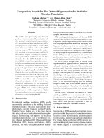
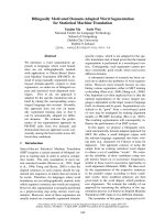
In MT, spurious ambiguity occurs both in regular
phrase-based systems (e.g., Koehn et al. (2003)),
where different segmentations lead to the same
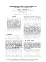
translation string (Figure 1), and in syntax-based
systems (e.g., Chiang (2007)), where different
derivation trees yield the same string (Figure 2).
In the Hiero system (Chiang, 2007) we are us-
ing, each string corresponds to about 115 distinct
derivations on average.
We use x to denote the input string, and D(x) to
consider the set of derivations then considered by
the system. Each derivation d ∈ D(x) yields some
translation string y = Y(d) in the target language.
We write D(x, y)
def
= {d ∈ D(x) : Y(d) = y} to
denote the set of all derivations that yield y. Thus,
the set of translations permitted by the model is
T(y)
def
= {y : D(x, y) = ∅} (or equivalently,
T(y)
def
= {Y(d) : d ∈ D(x)}). We write y
∗

for
the translation string that is actually output.
2.2 Maximum A Posterior (MAP) Decoding
For a given input sentence x, a decoding method
identifies a particular “best” output string y
∗
. The
maximum a posteriori (MAP) decision rule is
y
∗
= argmax
y∈T(x)
p(y | x) (1)
machine translation software
! " # $ % &
machine translation software
! " # $ % &
Figure 1: Segmentation ambiguity in phrase-based MT: two
different segmentations lead to the same translation string.
S->(! ", machine) S->(#$, translation) S->(%&, software)
S->(! ", machine)
#$
S->(%&, software)
S->(S0 S1, S0 S1)
S->(S0 S1, S0 S1)
S->(S0 #$ S1, S0 translation S1)
Figure 2: Tree ambiguity in syntax-based MT: two derivation
trees yield the same translation string.
(An alternative decision rule, minimum Bayes
risk (MBR), will be discussed in Section 4.)

To obtain p(y | x) above, we need to marginal-
ize over a nuisance variable, the derivation of y.
Therefore, the MAP decision rule becomes
y
∗
= argmax
y∈T(x)

d∈D(x,y)
p(y, d | x) (2)
where p(y, d | x) is typically derived from a log-
linear model as follows,
p(y, d | x) =
e
γ·s(x,y,d)
Z(x)
=
e
γ·s(x,y,d)

y,d
e
γ·s(x,y,d)
(3)
where γ is a scaling factor to adjust the sharp-
ness of the distribution, the score s(x, y, d) is a
learned linear combination of features of the triple
(x, y, d), and Z(x) is a normalization constant.
Note that p(y, d | x) = 0 if y = Y(d). Our deriva-
tion set D(x) is encoded in polynomial space, us-

ing a hypergraph or lattice.
3
However, both |D(x)|
and |T(x)| may be exponential in |x|. Since the
marginalization needs to be carried out for each
member of T(x), the decoding problem of (2)
turns out to be NP-hard,
4
as shown by Sima’an
(1996) for a similar problem.
3
A hypergraph is analogous to a parse forest (Huang and
Chiang, 2007). (A finite-state lattice is a special case.) It can
be used to encode exponentially many hypotheses generated
by a phrase-based MT system (e.g., Koehn et al. (2003)) or a
syntax-based MT system (e.g., Chiang (2007)).
4
Note that the marginalization for a particular y would be
tractable; it is used at training time in certain training objec-
tive functions, e.g., maximizing the conditional likelihood of
a reference translation (Blunsom et al., 2008).
594
2.3 Viterbi Approximation
To approximate the intractable decoding problem
of (2), most MT systems (Koehn et al., 2003; Chi-
ang, 2007) use a simple Viterbi approximation,
y
∗
= argmax
y∈T(x)

p
Viterbi
(y | x) (4)
= argmax
y∈T(x)
max
d∈D(x,y)
p(y, d | x) (5)
= Y

argmax
d∈D(x)
p(y, d | x)

(6)
Clearly, (5) replaces the sum in (2) with a max.
In other words, it approximates the probability of
a translation string by the probability of its most-
probable derivation. (5) is found quickly via (6).
The Viterbi approximation is simple and tractable,
but it ignores most derivations.
2.4 N-best Approximation (or Crunching)
Another popular approximation enumerates the N
best derivations in D(x), a set that we call ND(x).
Modifying (2) to sum over only these derivations
is called crunching by May and Knight (2006):
y
∗
= argmax
y∈T(x)

p
crunch
(y | x) (7)
= argmax
y∈T(x)

d∈D(x,y)∩ND(x)
p(y, d | x)
3 Variational Approximate Decoding
The Viterbi and crunching methods above approx-
imate the intractable decoding of (2) by ignor-
ing most of the derivations. In this section, we
will present a novel variational approximation,
which considers all the derivations but still allows
tractable decoding.
3.1 Approximate Inference
There are several popular approaches to approxi-
mate inference when exact inference is intractable
(Bishop, 2006). Stochastic techniques such as
Markov Chain Monte Carlo are exact in the limit
of infinite runtime, but tend to be too slow for large
problems. By contrast, deterministic variational
methods (Jordan et al., 1999), including message-
passing (Minka, 2005), are inexact but scale up
well. They approximate the original intractable
distribution with one that factorizes better or has
a specific parametric form (e.g., Gaussian).
In our work, we use a fast variational method.
Variational methods generally work as follows.
When exact inference under a complex model p

is intractable, one can approximate the posterior
p(y | x) by a tractable model q(y), where q ∈ Q is
chosen to minimize some information loss such as
the KL divergence KL(p  q). The simpler model
q can then act as a surrogate for p during inference.
3.2 Variational Decoding for MT
For each input sentence x, we assume that a base-
line MT system generates a hypergraph HG(x)
that compactly encodes the derivation set D(x)
along with a score for each d ∈ D(x),
5
which we
interpret as p(y, d | x) (or proportional to it). For
any single y ∈ T(x), it would be tractable using
HG(x) to compute p(y | x) =

d
p(y, d | x).
However, as mentioned, it is intractable to find
argmax
y
p(y | x) as required by the MAP de-
coding (2), so we seek an approximate distribution
q(y) ≈ p(y | x).
6
For a fixed x, we seek a distribution q ∈ Q that
minimizes the KL divergence from p to q (both
regarded as distributions over y):
7
q

∗
= argmin
q∈Q
KL(p  q) (8)
= argmin
q∈Q

y∈T(x)
(p log p − p log q) (9)
= argmax
q∈Q

y∈T(x)
p log q (10)
So far, in order to approximate the intractable
optimization problem (2), we have defined an-
other optimization problem (10). If computing
p(y | x) during decoding is computationally in-
tractable, one might wonder if the optimization
problem (10) is any simpler. We will show this is
the case. The trick is to parameterize q as a fac-
torized distribution such that the estimation of q
∗
and decoding using q
∗
are both tractable through
efficient dynamic programs. In the next three sub-
sections, we will discuss the parameterization, es-
timation, and decoding, respectively.
3.2.1 Parameterization of q

In (10), Q is a family of distributions. If we se-
lect a large family Q, we can allow more com-
plex distributions, so that q
∗
will better approxi-
mate p. If we select a smaller family Q, we can
5
The baseline system may return a pruned hypergraph,
which has the effect of pruning D(x) and T(x) as well.
6
Following the convention in describing variational infer-
ence, we write q(y) instead of q(y | x), even though q(y)
always depends on x implicitly.
7
To avoid clutter, we denote p(y | x) by p, and q(y) by q.
We drop p log p from (9) because it is constant with respect
to q. We then flip the sign and change argmin to argmax.
595
guarantee that q
∗
will have a simple form with
many conditional independencies, so that q
∗
(y)
and y
∗
= argmax
y
q
∗

(y) are easier to compute.
Since each q(y) is a distribution over output
strings, a natural choice for Q is the family of
n-gram models. To obtain a small KL diver-
gence (8), we should make n as large as possible.
In fact, q
∗
→ p as n → ∞. Of course, this last
point also means that our computation becomes
intractable as n → ∞.
8
However, if p(y | x) is de-
fined by a hypergraph HG(x) whose structure ex-
plicitly incorporates an m-gram language model,
both training and decoding will be efficient when
m ≥ n. We will give algorithms for this case that
are linear in the size of HG(x).
9
Formally, each q ∈ Q takes the form
q(y) =

w∈W
q(r(w) | h(w))
c
w
(y)
(11)
where W is a set of n-gram types. Each w ∈ W is
an n-gram, which occurs c
w

(y) times in the string
y, and w may be divided into an (n − 1)-gram
prefix h(w) (the history) and a 1-gram suffix r(w)
(the rightmost or current word).
8
Blunsom et al. (2008) effectively do take n = ∞, by
maintaining the whole translation string in the dynamic pro-
gramming state. They alleviate the computation cost some-
how by using aggressive beam pruning, which might be sen-
sible for their relatively small task (e.g., input sentences of
< 10 words). But, we are interested in improving the perfor-
mance for a large-scale system, and thus their method is not
a viable solution. Moreover, we observe in our experiments
that using a larger n does not improve much over n = 2.
9
A reviewer asks about the interaction with backed-off
language models. The issue is that the most compact finite-
state representations of these (Allauzen et al., 2003), which
exploit backoff structure, are not purely m-gram for any
m. They yield more compact hypergraphs (Li and Khudan-
pur, 2008), but unfortunately those hypergraphs might not be
treatable by Fig. 4—since where they back off to less than an
n-gram, e is not informative enough for line 8 to find w.
We sketch a method that works for any language model
given by a weighted FSA, L. The variational family Q can
be specified by any deterministic weighted FSA, Q, with
weights parameterized by φ. One seeks φ to minimize (8).
Intersect HG(x) with an “unweighted” version of Q in
which all arcs have weight 1, so that Q does not prefer
any string to another. By lifting weights into an expectation

semiring (Eisner, 2002), it is then possible to obtain expected
transition counts in Q (where the expectation is taken under
p), or other sufficient statistics needed to estimate φ.
This takes only time O(|HG(x)|) when L is a left-to-right
refinement of Q (meaning that any two prefix strings that
reach the same state in L also reach the same state in Q),
for then intersecting L or HG(x) with Q does not split any
states. That is the case when L and Q are respectively pure
m-gram and n-gram models with m ≥ n, as assumed in (12)
and Figure 4. It is also the case when Q is a pure n-gram
model and L is constructed not to back off beyond n-grams;
or when the variational family Q is defined by deliberately
taking the FSA Q to have the same topology as L.
The parameters that specify a particular q ∈ Q
are the (normalized) conditional probability distri-
butions q(r(w) | h(w)). We will now see how to
estimate these parameters to approximate p(· | x)
for a given x at test time.
3.2.2 Estimation of q
∗
Note that the objective function (8)–(10) asks us to
approximate p as closely as possible, without any
further smoothing. (It is assumed that p is already
smoothed appropriately, having been constructed
from channel and language models that were esti-
mated with smoothing from finite training data.)
In fact, if p were the empirical distribution over
strings in a training corpus, then q
∗
of (10) is just

the maximum-likelihood n-gram model—whose
parameters, trivially, are just unsmoothed ratios of
the n-gram and (n−1)-gram counts in the training
corpus. That is, q
∗
(r(w) | h(w)) =
c(w)
c(h(w))
.
Our actual job is exactly the same, except that p
is specified not by a corpus but by the hypergraph
HG(x). The only change is that the n-gram counts
¯c(w) are no longer integers from a corpus, but are
expected counts under p:
10
q
∗
(r(w) | h(w)) =
¯c(w)
¯c(h(w))
= (12)

y
c
w
(y)p(y | x)

y
c
h(w)

(y)p(y | x)
=

y,d
c
w
(y)p(y, d | x)

y,d
c
h(w)
(y)p(y, d | x)
Now, the question is how to efficiently compute
(12) from the hypergraph HG(x). To develop the
intuition, we first present a brute-force algorithm
in Figure 3. The algorithm is brute-force since
it first needs to unpack the hypergraph and enu-
merate each possible derivation in the hypergraph
(see line 1), which is computationally intractable.
The algorithm then enumerates each n-gram and
(n − 1)-gram in y and accumulates its soft count
into the expected count, and finally obtains the pa-
rameters of q
∗
by taking count ratios via (12).
Figure 4 shows an efficient version that exploits
the packed-forest structure of HG(x) in com-
puting the expected counts. Specifically, it first
runs the inside-outside procedure, which annotates
each node (say v) with both an inside weight β(v)

and an outside weight α(v). The inside-outside
also finds Z(x), the total weight of all derivations.
With these weights, the algorithm then explores
the hypergraph once more to collect the expected
10
One can prove (12) via Lagrange multipliers, with q
∗
(· |
h) constrained to be a normalized distribution for each h.
596
Brute-Force-MLE(HG(x ))
1 for y, d in HG(x) ✄ each derivation
2 for
w
in y ✄ each n-gram type
3 ✄ accumulate soft count
4 ¯c(w) + = c
w
(y) · p(y, d | x)
5 ¯c(h(w)) + = c
w
(y) · p(y, d | x)
6 q
∗
← MLE using formula (12)
7 return q
∗
Figure 3: Brute-force estimation of q
∗
.

Dynamic-Programming-MLE(HG(x ))
1 run inside-outside on the hypergraph HG(x)
2 for
v
in HG(x) ✄ each node
3 for
e
∈ B(v) ✄ each incoming hyperedge
4 c
e
← p
e
· α(v)/Z(x)
5 for
u
∈ T (e) ✄ each antecedent node
6 c
e
← c
e
· β(u)
7 ✄ accumulate soft count
8 for
w
in e ✄ each n-gram type
9 ¯c(w) + = c
w
(e) · c
e
10 ¯c(h(w)) + = c

w
(e) · c
e
11 q
∗
← MLE using formula (12)
12 return q
∗
Figure 4: Dynamic programming estimation of q
∗
. B(v) rep-
resents the set of incoming hyperedges of node v; p
e
repre-
sents the weight of the hyperedge e itself; T (e) represents
the set of antecedent nodes of hyperedge e. Please refer to
the text for the meanings of other notations.
counts. For each hyperedge (say e), it first gets the
posterior weight c
e
(see lines 4-6). Then, for each
n-gram type (say w), it increments the expected
count by c
w
(e) · c
e
, where c
w
(e) is the number of
copies of n-gram w that are added by hyperedge

e, i.e., that appear in the yield of e but not in the
yields of any of its antecedents u ∈ T (e).
While there may be exponentially many deriva-
tions, the hypergraph data structure represents
them in polynomial space by allowing multiple
derivations to share subderivations. The algorithm
of Figure 4 may be run over this packed forest
in time O(|HG(x)|) where |HG(x)| is the hyper-
graph’s size (number of hyperedges).
3.2.3 Decoding with q
∗
When translating x at runtime, the q
∗
constructed
from HG(x) will be used as a surrogate for p dur-
ing decoding. We want its most probable string:
y
∗
= argmax
y
q
∗
(y) (13)
Since q
∗
is an n-gram model, finding y
∗
is equiv-
alent to a shortest-path problem in a certain graph
whose edges correspond to n-grams (weighted

with negative log-probabilities) and whose ver-
tices correspond to (n − 1)-grams.
However, because q
∗
only approximates p, y
∗
of
(13) may be locally appropriate but globally inade-
quate as a translation of x. Observe, e.g., that an n-
gram model q
∗
(y) will tend to favor short strings
y, regardless of the length of x. Suppose x = le
chat chasse la souris (“the cat chases the mouse”)
and q
∗
is a bigram approximation to p(y | x). Pre-
sumably q
∗
(the | START), q
∗
(mouse | the), and
q
∗
(END | mouse) are all large in HG(x). So the
most probable string y
∗
under q
∗
may be simply

“the mouse,” which is short and has a high proba-
bility but fails to cover x.
Therefore, a better way of using q
∗
is to restrict
the search space to the original hypergraph, i.e.:
y
∗
= argmax
y∈T(x)
q
∗
(y) (14)
This ensures that y
∗
is a valid string in the origi-
nal hypergraph HG(x), which will tend to rule out
inadequate translations like “the mouse.”
If our sole objective is to get a good approxi-
mation to p(y | x), we should just use a single
n-gram model q
∗
whose order n is as large as pos-
sible, given computational constraints. This may
be regarded as favoring n-grams that are likely to
appear in the reference translation (because they
are likely in the derivation forest). However, in or-
der to score well on the BLEU metric for MT eval-
uation (Papineni et al., 2001), which gives partial
credit, we would also like to favor lower-order n-

grams that are likely to appear in the reference,
even if this means picking some less-likely high-
order n-grams. For this reason, it is useful to in-
terpolate different orders of variational models,
y
∗
= argmax
y∈T(x)

n
θ
n
· log q
∗
n
(y) (15)
where n may include the value of zero, in which
case log q
∗
0
(y)
def
= |y|, corresponding to a conven-
tional word penalty feature. In the geometric inter-
polation above, the weight θ
n
controls the relative
veto power of the n-gram approximation and can
be tuned using MERT (Och, 2003) or a minimum
risk procedure (Smith and Eisner, 2006).

Lastly, note that Viterbi and variational approx-
imation are different ways to approximate the ex-
act probability p(y | x), and each of them has
pros and cons. Specifically, Viterbi approxima-
tion uses the correct probability of one complete
597
derivation, but ignores most of the derivations in
the hypergraph. In comparison, the variational ap-
proximation considers all the derivations in the hy-
pergraph, but uses only aggregate statistics of frag-
ments of derivations. Therefore, it is desirable to
interpolate further with the Viterbi approximation
when choosing the final translation output:
11
y
∗
= argmax
y∈T(x)

n
θ
n
· log q
∗
n
(y)
+ θ
v
· log p
Viterbi

(y | x) (16)
where the first term corresponds to the interpolated
variational decoding of (15) and the second term
corresponds to the Viterbi decoding of (4).
12
As-
suming θ
v
> 0, the second term penalizes transla-
tions with no good derivation in the hypergraph.
13
For n ≤ m, any of these decoders (14)–
(16) may be implemented efficiently by using the
n-gram variational approximations q
∗
to rescore
HG(x)—preserving its hypergraph topology, but
modifying the hyperedge weights.
14
While the
original weights gave derivation d a score of
log p(d | x), the weights as modified for (16)
will give d a score of

n
θ
n
· log q
∗
n

(Y(d)) + θ
v
·
log p(d | x). We then find the best-scoring deriva-
tion and output its target yield; that is, we find
argmax
y∈T(x)
via Y(argmax
d∈D(x)
).
4 Variational vs. Min-Risk Decoding
In place of the MAP decoding, another commonly
used decision rule is minimum Bayes risk (MBR):
y
∗
= argmin
y
R(y) = argmin
y

y

l(y, y

)p(y

| x)
(17)
11
It would also be possible to interpolate with the N-best

approximations (see Section 2.4), with some complications.
12
Zens and Ney (2006) use a similar decision rule as here
and they also use posterior n-gram probabilities as feature
functions, but their model estimation and decoding are over
an N-best, which is trivial in terms of computation.
13
Already at (14), we explicitly ruled out translations y
having no derivation at all in the hypergraph. However,
suppose the hypergraph were very large (thanks to a large
or smoothed translation model and weak pruning). Then
(14)’s heuristic would fail to eliminate bad translations (“the
mouse”), since nearly every string y ∈ Σ
∗
would be derived
as a translation with at least a tiny probability. The “soft” ver-
sion (16) solves this problem, since unlike the “hard” (14), it
penalizes translations that appear only weakly in the hyper-
graph. As an extreme case, translations not in the hypergraph
at all are infinitely penalized (log p
Viterbi
(y) = log 0 =
−∞), making it natural for the decoder not to consider them,
i.e., to do only argmax
y∈T(x)
rather than argmax
y∈Σ
∗
.
14

One might also want to use the q
∗
n
or smoothed versions
of them to rescore additional hypotheses, e.g., hypotheses
proposed by other systems or by system combination.
where l(y, y

) represents the loss of y if the true
answer is y

, and the risk of y is its expected
loss.
15
Statistical decision theory shows MBR is
optimal if p(y

| x) is the true distribution, while
in practice p(y

| x) is given by a model at hand.
We now observe that our variational decoding
resembles the MBR decoding of Tromble et al.
(2008). They use the following loss function, of
which a linear approximation to BLEU (Papineni
et al., 2001) is a special case,
l(y, y

) = −(θ
0

|y| +

w∈N
θ
w
c
w
(y)δ
w
(y

)) (18)
where w is an n-gram type, N is a set of n-gram
types with n ∈ [1, 4], c
w
(y) is the number of oc-
currence of the n-gram w in y, and δ
w
(y

) is an
indicator function to check if y

contains at least
one occurrence of w. With the above loss func-
tion, Tromble et al. (2008) derive the MBR rule
16
y
∗
= argmax

y
(θ
0
|y| +

w∈N
θ
w
c
w
(y)g(w | x))
(19)
where g(w | x) is a specialized “posterior” proba-
bility of the n-gram w, and is defined as
g(w | x) =

y

δ
w
(y

)p(y

| x) (20)
Now, let us divide N , which contains n-gram
types of different n, into several subsets W
n
, each
of which contains only the n-grams with a given

length n. We can now rewrite (19) as follows,
y
∗
= argmax
y

n
θ
n
· g
n
(y | x) (21)
by assuming θ
w
= θ
|w|
and,
g
n
(y | x)=

|y| if n = 0

w∈W
n
g(w | x)c
w
(y) if n > 0
(22)
Clearly, their rule (21) has a quite similar form

to our rule (15), and we can relate (20) to (12) and
(22) to (11). This justifies the use of interpolation
in Section 3.2.3. However, there are several im-
portant differences. First, the n-gram “posterior”
of (20) is very expensive to compute. In fact, it re-
quires an intersection between each n-gram in the
lattice and the lattice itself, as is done by Tromble
15
The MBR becomes the MAP decision rule of (1) if a so-
called zero-one loss function is used: l(y, y

) = 0 if y = y

;
otherwise l(y, y

) = 1.
16
Note that Tromble et al. (2008) only consider MBR for a
lattice without hidden structures, though their method can be
in principle applied in a hypergraph with spurious ambiguity.
598
et al. (2008). In comparison, the optimal n-gram
probabilities of (12) can be computed using the
inside-outside algorithm, once and for all. Also,
g(w | x) of (20) is not normalized over the history
of w, while q
∗
(r(w) | h(w)) of (12) is. Lastly, the
definition of the n-gram model is different. While

the model (11) is a proper probabilistic model, the
function of (22) is simply an approximation of the
average n-gram precisions of y.
A connection between variational decoding and
minimum-risk decoding has been noted before
(e.g., Matsuzaki et al. (2005)), but the derivation
above makes the connection formal.
DeNero et al. (2009) concurrently developed
an alternate to MBR, called consensus decoding,
which is similar to ours in practice although moti-
vated quite differently.
5 Experimental Results
We report results using an open source MT toolkit,
called Joshua (Li et al., 2009), which implements
Hiero (Chiang, 2007).
5.1 Experimental Setup
We work on a Chinese to English translation task.
Our translation model was trained on about 1M
parallel sentence pairs (about 28M words in each
language), which are sub-sampled from corpora
distributed by LDC for the NIST MT evalua-
tion using a sampling method based on the n-
gram matches between training and test sets in
the foreign side. We also used a 5-gram lan-
guage model with modified Kneser-Ney smooth-
ing (Chen and Goodman, 1998), trained on a data
set consisting of a 130M words in English Giga-
word (LDC2007T07) and the English side of the
parallel corpora. We use GIZA++ (Och and Ney,
2000), a suffix-array (Lopez, 2007), SRILM (Stol-

cke, 2002), and risk-based deterministic annealing
(Smith and Eisner, 2006)
17
to obtain word align-
ments, translation models, language models, and
the optimal weights for combining these models,
respectively. We use standard beam-pruning and
cube-pruning parameter settings, following Chi-
ang (2007), when generating the hypergraphs.
The NIST MT’03 set is used to tune model
weights (e.g. those of (16)) and the scaling factor
17
We have also experimented with MERT (Och, 2003), and
found that the deterministic annealing gave results that were
more consistent across runs and often better.
Decoding scheme MT’04 MT’05
Viterbi 35.4 32.6
MBR (K=1000) 35.8 32.7
Crunching (N=10000) 35.7 32.8
Crunching+MBR (N=10000) 35.8 32.7
Variational (1to4gram+wp+vt) 36.6 33.5
Table 1: BLEU scores for Viterbi, Crunching, MBR, and vari-
ational decoding. All the systems improve significantly over
the Viterbi baseline (paired permutation test, p < 0.05). In
each column, we boldface the best result as well as all results
that are statistically indistinguishable from it. In MBR, K is
the number of unique strings. For Crunching and Crunch-
ing+MBR, N represents the number of derivations. On av-
erage, each string has about 115 distinct derivations. The
variational method “1to4gram+wp+vt” is our full interpola-

tion (16) of four variational n-gram models (“1to4gram”), the
Viterbi baseline (“vt”), and a word penalty feature (“wp”).
γ of (3),
18
and MT’04 and MT’05 are blind test-
sets. We will report results for lowercase BLEU-4,
using the shortest reference translation in comput-
ing brevity penalty.
5.2 Main Results
Table 1 presents the BLEU scores under Viterbi,
crunching, MBR, and variational decoding. Both
crunching and MBR show slight significant im-
provements over the Viterbi baseline; variational
decoding gives a substantial improvement.
The difference between MBR and Crunch-
ing+MBR lies in how we approximate the distri-
bution p(y

| x) in (17).
19
For MBR, we take
p(y

| x) to be proportional to p
Viterbi
(y

| x) if y

is among the K best distinct strings on that mea-

sure, and 0 otherwise. For Crunching+MBR, we
take p(y

| x) to be proportional to p
crunch
(y

| x),
which is based on the N best derivations.
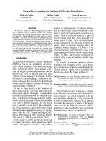
5.3 Results of Different Variational Decoding
Table 2 presents the BLEU results under different
ways in using the variational models, as discussed
in Section 3.2.3. As shown in Table 2a, decod-
ing with a single variational n-gram model (VM)
as per (14) improves the Viterbi baseline (except
the case with a unigram VM), though often not
statistically significant. Moreover, a bigram (i.e.,
“2gram”) achieves the best BLEU scores among
the four different orders of VMs.
The interpolation between a VM and a word
penalty feature (“wp”) improves over the unigram
18
We found the BLEU scores are not very sensitive to γ,
contrasting to the observations by Tromble et al. (2008).
19
We also restrict T(x) to {y : p(y | x) > 0}, using the
same approximation for p(y | x) as we did for p(y

| x).
599

(a) decoding with a single variational model
Decoding scheme MT’04 MT’05
Viterbi 35.4 32.6
1gram 25.9 24.5
2gram 36.1 33.4
3gram 36.0
∗
33.1
4gram 35.8
∗
32.9
(b) interpolation between a single variational
model and a word penalty feature
1gram+wp 29.7 27.7
2gram+wp 35.5 32.6
3gram+wp 36.1
∗
33.1
4gram+wp 35.7
∗
32.8
∗
(c) interpolation of a single variational model, the
Viterbi model, and a word penalty feature
1gram+wp+vt 35.6
∗
32.8
∗
2gram+wp+vt 36.5
∗

33.5
∗
3gram+wp+vt 35.8
∗
32.9
∗
4gram+wp+vt 35.6
∗
32.8
∗
(d) interpolation of several n-gram VMs, the
Viterbi model, and a word penalty feature
1to2gram+wp+vt 36.6
∗
33.6
∗
1to3gram+wp+vt 36.6
∗
33.5
∗
1to4gram+wp+vt 36.6
∗
33.5
∗
Table 2: BLEU scores under different variational decoders
discussed in Section 3.2.3. A star
∗
indicates a result that is
significantly better than Viterbi decoding (paired permutation
test, p < 0.05). We boldface the best system and all systems

that are not significantly worse than it. The brevity penalty
BP in BLEU is always 1, meaning that on average y
∗
is no
shorter than the reference translation, except for the “1gram”
systems in (a), which suffer from brevity penalties of 0.826
and 0.831.
VM dramatically, but does not improve higher-
order VMs (Table 2b). Adding the Viterbi fea-
ture (“vt”) into the interpolation further improves
the lower-order models (Table 2c), and all the im-
provements over the Viterbi baseline become sta-
tistically significant. At last, interpolation of sev-
eral variational models does not yield much fur-
ther improvement over the best previous model,
but makes the results more stable (Table 2d).
5.4 KL Divergence of Approximate Models
While the BLEU scores reported show the prac-
tical utility of the variational models, it is also
interesting to measure how well each individual
variational model q(y) approximates the distribu-
tion p(y | x). Ideally, the quality of approxima-
tion should be measured by the KL divergence
KL(p  q)
def
= H(p, q) − H(p), where the cross-
entropy H(p, q)
def
= −


y
p(y | x) log q(y), and
Measure H(p, ·) H
d
(p) H(p)
bits/word q
∗
1
q
∗
2
q
∗
3
q
∗
4
≈
MT’04 2.33 1.68 1.57 1.53 1.36 1.03
MT’05 2.31 1.69 1.58 1.54 1.37 1.04
Table 3: Cross-entropies H(p, q) achieved by various ap-
proximations q. The notation H denotes the sum of cross-
entropies of all test sentences, divided by the total number
of test words. A perfect approximation would achieve H(p),
which we estimate using the true H
d
(p) and a 10000-best list.
the entropy H(p)
def
= −


y
p(y | x) log p(y | x).
Unfortunately H(p) (and hence KL = H(p, q) −
H(p)) is intractable to compute. But, since H(p)
is the same for all q, we can simply use H(p, q)
to compare different models q. Table 3 reports the
cross-entropies H(p, q) for various models q.
We also report the derivational entropy
H
d
(p)
def
= −

d
p(d | x) log p(d | x).
20
From this,
we obtain an estimate of H(p) by observing that
the “gap” H
d
(p) − H(p) equals E
p(y)
[H(d | y)],
which we estimate from our 10000-best list.
Table 3 confirms that higher-order variational
models (drawn from a larger family Q) approxi-
mate p better. This is necessarily true, but it is
interesting to see that most of the improvement is

obtained just by moving from a unigram to a bi-
gram model. Indeed, although Table 3 shows that
better approximations can be obtained by using
higher-order models, the best BLEU score in Ta-
bles 2a and 2c was obtained by the bigram model.
After all, p cannot perfectly predict the reference
translation anyway, hence may not be worth ap-
proximating closely; but p may do a good job
of predicting bigrams of the reference translation,
and the BLEU score rewards us for those.
6 Conclusions and Future Work
We have successfully applied the general varia-
tional inference framework to a large-scale MT
task, to approximate the intractable problem of
MAP decoding in the presence of spurious am-
biguity. We also showed that interpolating vari-
ational models with the Viterbi approximation can
compensate for poor approximations, and that in-
terpolating them with one another can reduce the
Bayes risk and improve BLEU. Our empirical re-
sults improve the state of the art.
20
Both H(p, q) and H
d
(p) involve an expectation over ex-
ponentially many derivations, but they can be computed in
time only linear in the size of HG(x) using an expectation
semiring (Eisner, 2002). In particular, H(p, q) can be found
as −


d∈D(x)
p(d | x) log q(Y(d)).
600
Many interesting research directions remain
open. To approximate the intractable MAP de-
coding problem of (2), we can use different vari-
ational distributions other than the n-gram model
of (11). Interpolation with other models is also
interesting, e.g., the constituent model in Zhang
and Gildea (2008). We might also attempt to min-
imize KL(q  p) rather than KL(p  q), in order
to approximate the mode (which may be prefer-
able since we care most about the 1-best transla-
tion under p) rather than the mean of p (Minka,
2005). One could also augment our n-gram mod-
els with non-local string features (Rosenfeld et al.,
2001) provided that the expectations of these fea-
tures could be extracted from the hypergraph.
Variational inference can also be exploited to
solve many other intractable problems in MT (e.g.,
word/phrase alignment and system combination).
Finally, our method can be used for tasks beyond
MT. For example, it can be used to approximate
the intractable MAP decoding inherent in systems
using HMMs (e.g. speech recognition). It can also
be used to approximate a context-free grammar
with a finite state automaton (Nederhof, 2005).
References
Cyril Allauzen, Mehryar Mohri, and Brian Roark.
2003. Generalized algorithms for constructing sta-

tistical language models. In ACL, pages 40–47.
Christopher M. Bishop. 2006. Pattern recognition and
machine learning. Springer.
Phil Blunsom, Trevor Cohn, and Miles Osborne. 2008.
A discriminative latent variable model for statistical
machine translation. In ACL, pages 200–208.
Francisco Casacuberta and Colin De La Higuera. 2000.
Computational complexity of problems on proba-
bilistic grammars and transducers. In ICGI, pages
15–24.
Stanley F. Chen and Joshua Goodman. 1998. An em-
pirical study of smoothing techniques for language
modeling. Technical report.
David Chiang. 2007. Hierarchical phrase-based trans-
lation. Computational Linguistics, 33(2):201–228.
John DeNero, David Chiang, and Kevin Knight. 2009.
Fast consensus decoding over translation forests. In
ACL-IJCNLP.
Jason Eisner. 2002. Parameter estimation for proba-
bilistic finite-state transducers. In ACL, pages 1–8.
Joshua Goodman. 1996. Efficient algorithms for pars-
ing the DOP model. In EMNLP, pages 143–152.
Liang Huang and David Chiang. 2007. Forest rescor-
ing: Faster decoding with integrated language mod-
els. In ACL, pages 144–151.
M. I. Jordan, Z. Ghahramani, T. S. Jaakkola, and L. K.
Saul. 1999. An introduction to variational meth-
ods for graphical models. In Learning in Graphical
Models. MIT press.
Philipp Koehn, Franz Josef Och, and Daniel Marcu.

2003. Statistical phrase-based translation. In
NAACL, pages 48–54.
Zhifei Li and Sanjeev Khudanpur. 2008. A scalable
decoder for parsing-based machine translation with
equivalent language model state maintenance. In
ACL SSST, pages 10–18.
Zhifei Li, Chris Callison-Burch, Chris Dyer, Juri
Ganitkevitch, Sanjeev Khudanpur, Lane Schwartz,
Wren Thornton, Jonathan Weese, and Omar. Zaidan.
2009. Joshua: An open source toolkit for parsing-
based machine translation. In WMT09, pages 135–
139.
Adam Lopez. 2007. Hierarchical phrase-based trans-
lation with suffix arrays. In EMNLP-CoNLL, pages
976–985.
Takuya Matsuzaki, Yusuke Miyao, and Jun’ichi Tsujii.
2005. Probabilistic CFG with latent annotations. In
ACL, pages 75–82.
Jonathan May and Kevin Knight. 2006. A better n-best
list: practical determinization of weighted finite tree
automata. In NAACL, pages 351–358.
Tom Minka. 2005. Divergence measures and message
passing. In Microsoft Research Technical Report
(MSR-TR-2005-173). Microsoft Research.
Mark-Jan Nederhof. 2005. A general technique to
train language models on language models. Com-
put. Linguist., 31(2):173–186.
Franz Josef Och and Hermann Ney. 2000. Improved
statistical alignment models. In ACL, pages 440–
447.

Franz Josef Och. 2003. Minimum error rate training in
statistical machine translation. In ACL, pages 160–
167.
Kishore Papineni, Salim Roukos, Todd Ward, and Wei-
Jing Zhu. 2001. Bleu: a method for automatic eval-
uation of machine translation. In ACL, pages 311–
318.
Roni Rosenfeld, Stanley F. Chen, and Xiaojin Zhu.
2001. Whole-sentence exponential language mod-
els: A vehicle for linguistic-statistical integration.
Computer Speech and Language, 15(1).
Khalil Sima’an. 1996. Computational complexity
of probabilistic disambiguation by means of tree-
grammars. In COLING, pages 1175–1180.
David A. Smith and Jason Eisner. 2006. Minimum risk
annealing for training log-linear models. In ACL,
pages 787–794.
Andreas Stolcke. 2002. Srilm - an extensible language
modeling toolkit. In ICSLP, pages 901–904.
Roy Tromble, Shankar Kumar, Franz Och, and Wolf-
gang Macherey. 2008. Lattice Minimum Bayes-
Risk decoding for statistical machine translation. In
EMNLP, pages 620–629.
Richard Zens and Hermann Ney. 2006. N-gram poste-
rior probabilities for statistical machine translation.
In WMT06, pages 72–77.
Hao Zhang and Daniel Gildea. 2008. Efficient multi-
pass decoding for synchronous context free gram-
mars. In ACL, pages 209–217.
601