Báo cáo khoa học: "Learning Document-Level Semantic Properties from Free-text Annotations" pot

Proceedings of ACL-08: HLT, pages 263–271,
Columbus, Ohio, USA, June 2008.
c
2008 Association for Computational Linguistics
Learning Document-Level Semantic Properties from Free-text Annotations
S.R.K. Branavan Harr Chen Jacob Eisenstein Regina Barzilay
Computer Science and Artificial Intelligence Laboratory
Massachusetts Institute of Technology
{branavan, harr, jacobe, regina} @csail.mit.edu
Abstract
This paper demonstrates a new method for
leveraging free-text annotations to infer se-
mantic properties of documents. Free-text an-
notations are becoming increasingly abundant,
due to the recent dramatic growth in semi-
structured, user-generated online content. An
example of such content is product reviews,
which are often annotated by their authors
with pros/cons keyphrases such as “a real bar-
gain” or “good value.” To exploit such noisy
annotations, we simultaneously find a hid-
den paraphrase structure of the keyphrases, a
model of the document texts, and the underly-
ing semantic properties that link the two. This
allows us to predict properties of unannotated
documents. Our approach is implemented as
a hierarchical Bayesian model with joint in-
ference, which increases the robustness of the
keyphrase clustering and encourages the doc-
ument model to correlate with semantically
meaningful properties. We perform several

evaluations of our model, and find that it sub-
stantially outperforms alternative approaches.
1 Introduction
A central problem in language understanding is
transforming raw text into structured representa-
tions. Learning-based approaches have dramatically
increased the scope and robustness of this type of
automatic language processing, but they are typi-
cally dependent on large expert-annotated datasets,
which are costly to produce. In this paper, we show
how novice-generated free-text annotations avail-
able online can be leveraged to automatically infer
document-level semantic properties.
With the rapid increase of online content cre-
ated by end users, noisy free-text annotations have
pros/cons: great nutritional value
combines it all: an amazing product, quick and
friendly service, cleanliness, great nutrition
pros/cons: a bit pricey, healthy
is an awesome place to go if you are health con-
scious. They have some really great low calorie dishes
and they publish the calories and fat grams per serving.
Figure 1: Excerpts from online restaurant reviews with
pros/cons phrase lists. Both reviews discuss healthiness,
but use different keyphrases.
become widely available (Vickery and Wunsch-
Vincent, 2007; Sterling, 2005). For example, con-
sider reviews of consumer products and services.
Often, such reviews are annotated with keyphrase
lists of pros and cons. We would like to use these

keyphrase lists as training labels, so that the proper-
ties of unannotated reviews can be predicted. Hav-
ing such a system would facilitate structured access
and summarization of this data. However, novice-
generated keyphrase annotations are incomplete de-
scriptions of their corresponding review texts. Fur-
thermore, they lack consistency: the same under-
lying property may be expressed in many ways,
e.g., “healthy” and “great nutritional value” (see Fig-
ure 1). To take advantage of such noisy labels, a sys-
tem must both uncover their hidden clustering into
properties, and learn to predict these properties from
review text.
This paper presents a model that addresses both
problems simultaneously. We assume that both the
document text and the selection of keyphrases are
governed by the underlying hidden properties of the
document. Each property indexes a language model,
thus allowing documents that incorporate the same
263
property to share similar features. In addition, each
keyphrase is associated with a property; keyphrases
that are associated with the same property should
have similar distributional and surface features.
We link these two ideas in a joint hierarchical
Bayesian model. Keyphrases are clustered based
on their distributional and lexical properties, and a
hidden topic model is applied to the document text.
Crucially, the keyphrase clusters and document top-
ics are linked, and inference is performed jointly.

This increases the robustness of the keyphrase clus-
tering, and ensures that the inferred hidden topics
are indicative of salient semantic properties.
Our model is broadly applicable to many scenar-
ios where documents are annotated in a noisy man-
ner. In this work, we apply our method to a col-
lection of reviews in two categories: restaurants and
cell phones. The training data consists of review text
and the associated pros/cons lists. We then evaluate
the ability of our model to predict review properties
when the pros/cons list is hidden. Across a variety
of evaluation scenarios, our algorithm consistently
outperforms alternative strategies by a wide margin.
2 Related Work
Review Analysis Our approach relates to previous
work on property extraction from reviews (Popescu
et al., 2005; Hu and Liu, 2004; Kim and Hovy,
2006). These methods extract lists of phrases, which
are analogous to the keyphrases we use as input
to our algorithm. However, our approach is dis-
tinguished in two ways: first, we are able to pre-
dict keyphrases beyond those that appear verbatim
in the text. Second, our approach learns the rela-
tionships between keyphrases, allowing us to draw
direct comparisons between reviews.
Bayesian Topic Modeling One aspect of our
model views properties as distributions over words
in the document. This approach is inspired by meth-
ods in the topic modeling literature, such as Latent
Dirichlet Allocation (LDA) (Blei et al., 2003), where

topics are treated as hidden variables that govern the
distribution of words in a text. Our algorithm ex-
tends this notion by biasing the induced hidden top-
ics toward a clustering of known keyphrases. Tying
these two information sources together enhances the
robustness of the hidden topics, thereby increasing
the chance that the induced structure corresponds to
semantically meaningful properties.
Recent work has examined coupling topic mod-
els with explicit supervision (Blei and McAuliffe,
2007; Titov and McDonald, 2008). However, such
approaches assume that the documents are labeled
within a predefined annotation structure, e.g., the
properties of food, ambiance, and service for restau-
rants. In contrast, we address free-text annotations
created by end users, without known semantic prop-
erties. Rather than requiring a predefined annotation
structure, our model infers one from the data.
3 Problem Formulation
We formulate our problem as follows. We assume
a dataset composed of documents with associated
keyphrases. Each document may be marked with
multiple keyphrases that express unseen semantic
properties. Across the entire collection, several
keyphrases may express the same property. The
keyphrases are also incomplete — review texts of-
ten express properties that are not mentioned in their
keyphrases. At training time, our model has access
to both text and keyphrases; at test time, the goal is
to predict the properties supported by a previously

unseen document. We can then use this property list
to generate an appropriate set of keyphrases.
4 Model Description
Our approach leverages both keyphrase clustering
and distributional analysis of the text in a joint, hi-
erarchical Bayesian model. Keyphrases are drawn
from a set of clusters; words in the documents are
drawn from language models indexed by a set of
topics, where the topics correspond to the keyphrase
clusters. Crucially, we bias the assignment of hid-
den topics in the text to be similar to the topics rep-
resented by the keyphrases of the document, but we
permit some words to be drawn from other topics
not represented by the keyphrases. This flexibility in
the coupling allows the model to learn effectively in
the presence of incomplete keyphrase annotations,
while still encouraging the keyphrase clustering to
cohere with the topics supported by the text.
We train the model on documents annotated with
keyphrases. During training, we learn a hidden
topic model from the text; each topic is also asso-
264
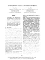
ψ – keyphrase cluster model
x – keyphrase cluster assignment
s – keyphrase similarity values
h – document keyphrases
η – document keyphrase topics
λ – probability of selecting η instead of φ
c – selects between η and φ for word topics
φ – document topic model

z – word topic assignment
θ – language models of each topic
w – document words
ψ ∼ Dirichlet(ψ
0
)
x
ℓ
∼ Multinomial(ψ)
s
ℓ,ℓ
′
∼

Beta(α
=
) if x
ℓ
= x
ℓ
′
Beta(α
=
) otherwise
η
d
= [η
d,1
. . . η
d,K

]
T
where
η
d,k
∝

1 if x
ℓ
= k for any l ∈ h
d
0 otherwise
λ ∼ Beta(λ
0
)
c
d,n
∼ Bernoulli(λ)
φ
d
∼ Dirichlet(φ
0
)
z
d,n
∼

Multinomial(η
d
) if c

d,n
= 1
Multinomial(φ
d
) otherwise
θ
k
∼ Dirichlet(θ
0
)
w
d,n
∼ Multinomial(θ
z
d,n
)
Figure 2: The plate diagram for our model. Shaded circles denote observed variables, and squares denote hyper
parameters. The dotted arrows indicate that η is constructed deterministically from x and h.
ciated with a cluster of keyphrases. At test time,
we are presented with documents that do not con-
tain keyphrase annotations. The hidden topic model
of the review text is used to determine the proper-
ties that a document as a whole supports. For each
property, we compute the proportion of the docu-
ment’s words assigned to it. Properties with propor-
tions above a set threshold (tuned on a development
set) are predicted as being supported.
4.1 Keyphrase Clustering
One of our goals is to cluster the keyphrases, such
that each cluster corresponds to a well-defined prop-

erty. We represent each distinct keyphrase as a vec-
tor of similarity scores computed over the set of
observed keyphrases; these scores are represented
by s in Figure 2, the plate diagram of our model.
1
Modeling the similarity matrix rather than the sur-
1
We assume that similarity scores are conditionally inde-
pendent given the keyphrase clustering, though the scores are
in fact related. Such simplifying assumptions have been previ-
ously used with success in NLP (e.g., Toutanova and Johnson,
2007), though a more theoretically sound treatment of the sim-
ilarity matrix is an area for future research.
face forms allows arbitrary comparisons between
keyphrases, e.g., permitting the use of both lexical
and distributional information. The lexical com-
parison is based on the cosine similarity between
the keyphrase words. The distributional similar-
ity is quantified in terms of the co-occurrence of
keyphrases across review texts. Our model is inher-
ently capable of using any arbitrary source of simi-
larity information; for a discussion of similarity met-
rics, see Lin (1998).
4.2 Document-level Distributional Analysis
Our analysis of the document text is based on proba-
bilistic topic models such as LDA (Blei et al., 2003).
In the LDA framework, each word is generated from
a language model that is indexed by the word’s topic
assignment. Thus, rather than identifying a single
topic for a document, LDA identifies a distribution

over topics.
Our word model operates similarly, identifying a
topic for each word, written as z in Figure 2. To
tie these topics to the keyphrases, we deterministi-
cally construct a document-specific topic distribu-
265
tion from the clusters represented by the document’s
keyphrases — this is η in the figure. η assigns equal
probability to all topics that are represented in the
keyphrases, and a small smoothing probability to
other topics.
As noted above, properties may be expressed in
the text even when no related keyphrase appears. For
this reason, we also construct a document-specific
topic distribution φ. The auxiliary variable c indi-
cates whether a given word’s topic is drawn from
the set of keyphrase clusters, or from this topic dis-
tribution.
4.3 Generative Process
In this section, we describe the underlying genera-
tive process more formally.
First we consider the set of all keyphrases ob-
served across the entire corpus, of which there are
L. We draw a multinomial distribution ψ over the K
keyphrase clusters from a symmetric Dirichlet prior
ψ
0
. Then for the ℓ
th
keyphrase, a cluster assign-

ment x
ℓ
is drawn from the multinomial ψ. Finally,
the similarity matrix s ∈ [0, 1]
L×L
is constructed.
Each entry s
ℓ,ℓ
′
is drawn independently, depending
on the cluster assignments x
ℓ
and x
ℓ
′
. Specifically,
s
ℓ,ℓ
′
is drawn from a Beta distribution with parame-
ters α
=
if x
ℓ
= x
ℓ
′
and α
=
otherwise. The parame-

ters α
=
linearly bias s
ℓ,ℓ
′
towards one (Beta(α
=
) ≡
Beta(2, 1)), and the parameters α
=
linearly bias s
ℓ,ℓ
′
towards zero (Beta(α
=
) ≡ Beta(1, 2)).
Next, the words in each of the D documents
are generated. Document d has N
d
words; z
d,n
is
the topic for word w
d,n
. These latent topics are
drawn either from the set of clusters represented by
the document’s keyphrases, or from the document’s
topic model φ
d
. We deterministically construct a

document-specific keyphrase topic model η
d
, based
on the keyphrase cluster assignments x and the ob-
served keyphrases h
d
. The multinomial η
d
assigns
equal probability to each topic that is represented by
a phrase in h
d
, and a small probability to other top-
ics.
As noted earlier, a document’s text may support
properties that are not mentioned in its observed
keyphrases. For that reason, we draw a document
topic multinomial φ
d
from a symmetric Dirichlet
prior φ
0
. The binary auxiliary variable c
d,n
deter-
mines whether the word’s topic is drawn from the
keyphrase model η
d
or the document topic model
φ

d
. c
d,n
is drawn from a weighted coin flip, with
probability λ; λ is drawn from a Beta distribution
with prior λ
0
. We have z
d,n
∼ η
d
if c
d,n
= 1,
and z
d,n
∼ φ
d
otherwise. Finally, the word w
d,n
is drawn from the multinomial θ
z
d,n
, where z
d,n
in-
dexes a topic-specific language model. Each of the
K language models θ
k
is drawn from a symmetric

Dirichlet prior θ
0
.
5 Posterior Sampling
Ultimately, we need to compute the model’s poste-
rior distribution given the training data. Doing so
analytically is intractable due to the complexity of
the model, but sampling-based techniques can be
used to estimate the posterior. We employ Gibbs
sampling, previously used in NLP by Finkel et al.
(2005) and Goldwater et al. (2006), among others.
This technique repeatedly samples from the condi-
tional distributions of each hidden variable, eventu-
ally converging on a Markov chain whose stationary
distribution is the posterior distribution of the hid-
den variables in the model (Gelman et al., 2004).
We now present sampling equations for each of the
hidden variables in Figure 2.
The prior over keyphrase clusters ψ is sampled
based on hyperprior ψ
0
and keyphrase cluster as-
signments x. We write p(ψ | . . .) to mean the prob-
ability conditioned on all the other variables.
p(ψ | . . .) ∝ p(ψ | ψ
0
)p(x | ψ),
= p(ψ | ψ
0
)

L

ℓ
p(x
ℓ
| ψ)
= Dir(ψ; ψ
0
)
L

ℓ
Mul(x
ℓ
; ψ)
= Dir(ψ; ψ
′
),
where ψ
′
i
= ψ
0
+ count(x
ℓ
= i). This update rule
is due to the conjugacy of the multinomial to the
Dirichlet distribution. The first line follows from
Bayes’ rule, and the second line from the conditional
independence of each keyphrase assignment x

ℓ
from
the others, given ψ.
φ
d
and θ
k
are resampled in a similar manner:
p(φ
d
| . . .) ∝ Dir(φ
d
; φ
′
d
),
p(θ
k
| . . .) ∝ Dir(θ
k
; θ
′
k
),
266
p(x
ℓ
| . . .) ∝ p(x
ℓ
| ψ)p(s | x

ℓ
, x
−ℓ
, α)p(z | η, ψ, c)
∝ p(x
ℓ
| ψ)



ℓ
′
=ℓ
p(s
ℓ,ℓ
′
| x
ℓ
, x
ℓ
′
, α)




D

d


c
d,n
=1
p(z
d,n
| η
d
)


= Mul(x
ℓ
; ψ)



ℓ
′
=ℓ
Beta(s
ℓ,ℓ
′
; α
x
ℓ
,x
ℓ
′
)





D

d

c
d,n
=1
Mul(z
d,n
; η
d
)


Figure 3: The resampling equation for the keyphrase cluster assignments.
where φ
′
d,i
= φ
0
+ count(z
d,n
= i ∧ c
d,n
= 0)
and θ
′

k,i
= θ
0
+

d
count(w
d,n
= i ∧ z
d,n
= k). In
building the counts for φ
′
d,i
, we consider only cases
in which c
d,n
= 0, indicating that the topic z
d,n
is
indeed drawn from the document topic model φ
d
.
Similarly, when building the counts for θ
′
k
, we con-
sider only cases in which the word w
d,n
is drawn

from topic k.
To resample λ, we employ the conjugacy of the
Beta prior to the Bernoulli observation likelihoods,
adding counts of c to the prior λ
0
.
p(λ | . . .) ∝ Beta(λ; λ
′
),
where λ
′
= λ
0
+


d
count(c
d,n
= 1)

d
count(c
d,n
= 0)

.
The keyphrase cluster assignments are repre-
sented by x, whose sampling distribution depends
on ψ, s, and z, via η. The equation is shown in Fig-

ure 3. The first term is the prior on x
ℓ
. The second
term encodes the dependence of the similarity ma-
trix s on the cluster assignments; with slight abuse of
notation, we write α
x
ℓ
,x
ℓ
′
to denote α
=
if x
ℓ
= x
ℓ
′
,
and α
=
otherwise. The third term is the dependence
of the word topics z
d,n
on the topic distribution η
d
.
We compute the final result of Figure 3 for each pos-
sible setting of x
ℓ

, and then sample from the normal-
ized multinomial.
The word topics z are sampled according to
keyphrase topic distribution η
d
, document topic dis-
tribution φ
d
, words w, and auxiliary variables c:
p(z
d,n
| . . .)
∝ p(z
d,n
| φ
d
, η
d
, c
d,n
)p(w
d,n
| z
d,n
, θ)
=

Mul(z
d,n
; η

d
)Mul(w
d,n
; θ
z
d,n
) if c
d,n
= 1,
Mul(z
d,n
; φ
d
)Mul(w
d,n
; θ
z
d,n
) otherwise.
As with x
ℓ
, each z
d,n
is sampled by computing
the conditional likelihood of each possible setting
within a constant of proportionality, and then sam-
pling from the normalized multinomial.
Finally, we sample each auxiliary variable c
d,n
,

which indicates whether the hidden topic z
d,n
is
drawn from η
d
or φ
d
. The conditional probability
for c
d,n
depends on its prior λ and the hidden topic
assignments z
d,n
:
p(c
d,n
| . . .)
∝ p(c
d,n
| λ)p(z
d,n
| η
d
, φ
d
, c
d,n
)
=


Bern(c
d,n
; λ)Mul(z
d,n
; η
d
) if c
d,n
= 1,
Bern(c
d,n
; λ)Mul(z
d,n
; φ
d
) otherwise.
We compute the likelihood of c
d,n
= 0 and c
d,n
= 1
within a constant of proportionality, and then sample
from the normalized Bernoulli distribution.
6 Experimental Setup
Data Sets We evaluate our system on reviews from
two categories, restaurants and cell phones. These
reviews were downloaded from the popular Epin-
ions
2
website. Users of this website evaluate prod-

ucts by providing both a textual description of their
opinion, as well as concise lists of keyphrases (pros
and cons) summarizing the review. The statistics of
this dataset are provided in Table 1. For each of
the categories, we randomly selected 50%, 15%, and
35% of the documents as training, development, and
test sets, respectively.
Manual analysis of this data reveals that authors
often omit properties mentioned in the text from
the list of keyphrases. To obtain a complete gold
2
/>267
Restaurants Cell Phones
# of reviews 3883 1112
Avg. review length 916.9 1056.9
Avg. keyphrases / review 3.42 4.91
Table 1: Statistics of the reviews dataset by category.
standard, we hand-annotated a subset of the reviews
from the restaurant category. The annotation effort
focused on eight commonly mentioned properties,
such as those underlying the keyphrases “pleasant
atmosphere” and “attentive staff.” Two raters anno-
tated 160 reviews, 30 of which were annotated by
both. Cohen’s kappa, a measure of interrater agree-
ment ranging from zero to one, was 0.78 for this sub-
set, indicating high agreement (Cohen, 1960).
Each review was annotated with 2.56 properties
on average. Each manually-annotated property cor-
responded to an average of 19.1 keyphrases in the
restaurant data, and 6.7 keyphrases in the cell phone

data. This supports our intuition that a single se-
mantic property may be expressed using a variety of
different keyphrases.
Training Our model needs to be provided with the
number of clusters K. We set K large enough for the
model to learn effectively on the development set.
For the restaurant data — where the gold standard
identified eight semantic properties — we set K to
20, allowing the model to account for keyphrases not
included in the eight most common properties. For
the cell phones category, we set K to 30.
To improve the model’s convergence rate, we per-
form two initialization steps for the Gibbs sampler.
First, sampling is done only on the keyphrase clus-
tering component of the model, ignoring document
text. Second, we fix this clustering and sample the
remaining model parameters. These two steps are
run for 5,000 iterations each. The full joint model
is then sampled for 100,000 iterations. Inspection
of the parameter estimates confirms model conver-
gence. On a 2GHz dual-core desktop machine, a
multi-threaded C++ implementation of model train-
ing takes about two hours for each dataset.
Inference The final point estimate used for test-
ing is an average (for continuous variables) or a
mode (for discrete variables) over the last 1,000
Gibbs sampling iterations. Averaging is a heuris-
tic that is applicable in our case because our sam-
ple histograms are unimodal and exhibit low skew.
The model usually works equally well using single-

sample estimates, but is more prone to estimation
noise.
As previously mentioned, we convert word topic
assignments to document properties by examining
the proportion of words supporting each property. A
threshold for this proportion is set for each property
via the development set.
Evaluation Our first evaluation examines the ac-
curacy of our model and the baselines by compar-
ing their output against the keyphrases provided by
the review authors. More specifically, the model
first predicts the properties supported by a given re-
view. We then test whether the original authors’
keyphrases are contained in the clusters associated
with these properties.
As noted above, the authors’ keyphrases are of-
ten incomplete. To perform a noise-free compari-
son, we based our second evaluation on the man-
ually constructed gold standard for the restaurant
category. We took the most commonly observed
keyphrase from each of the eight annotated proper-
ties, and tested whether they are supported by the
model based on the document text.
In both types of evaluation, we measure the
model’s performance using precision, recall, and F-
score. These are computed in the standard manner,
based on the model’s keyphrase predictions com-
pared against the corresponding references. The
sign test was used for statistical significance test-
ing (De Groot and Schervish, 2001).

Baselines To the best of our knowledge, this task
not been previously addressed in the literature. We
therefore consider five baselines that allow us to ex-
plore the properties of this task and our model.
Random: Each keyphrase is supported by a doc-
ument with probability of one half. This baseline’s
results are computed (in expectation) rather than ac-
tually run. This method is expected to have a recall
of 0.5, because in expectation it will select half of
the correct keyphrases. Its precision is the propor-
tion of supported keyphrases in the test set.
Phrase in text: A keyphrase is supported by a doc-
ument if it appears verbatim in the text. Because of
this narrow requirement, precision should be high
whereas recall will be low.
268
Restaurants Restaurants Cell Phones
gold standard annotation free-text annotation free-text annotation
Recall Prec. F-score Recall Prec. F-score Recall Prec. F-score
Random 0.500 0.300 ∗ 0.375 0.500 0.500 ∗ 0.500 0.500 0.489 ∗ 0.494
Phrase in text 0.048 0.500 ∗ 0.087 0.078 0.909 ∗ 0.144 0.171 0.529 ∗ 0.259
Cluster in text 0.223 0.534 0.314 0.517 0.640 ∗ 0.572 0.829 0.547 0.659
Phrase classifier 0.028 0.636 ∗ 0.053 0.068 0.963 ∗ 0.126 0.029 0.600 ∗ 0.055
Cluster classifier 0.113 0.622 ⋄ 0.192 0.255 0.907 ∗ 0.398 0.210 0.759 0.328
Our model 0.625 0.416 0.500 0.901 0.652 0.757 0.886 0.585 0.705
Our model + gold clusters 0.582 0.398 0.472 0.795 0.627 ∗ 0.701 0.886 0.520 ⋄ 0.655
Table 2: Comparison of the property predictions made by our model and the baselines in the two categories as evaluated
against the gold and free-text annotations. Results for our model using the fixed, manually-created gold clusterings are
also shown. The methods against which our model has significantly better results on the sign test are indicated with a
∗ for p <= 0.05, and ⋄ for p <= 0.1.

Cluster in text: A keyphrase is supported by a
document if it or any of its paraphrases appears in
the text. Paraphrasing is based on our model’s clus-
tering of the keyphrases. The use of paraphrasing
information enhances recall at the potential cost of
precision, depending on the quality of the clustering.
Phrase classifier: Discriminative classifiers are
trained for each keyphrase. Positive examples are
documents that are labeled with the keyphrase;
all other documents are negative examples. A
keyphrase is supported by a document if that
keyphrase’s classifier returns positive.
Cluster classifier: Discriminative classifiers are
trained for each cluster of keyphrases, using our
model’s clustering. Positive examples are docu-
ments that are labeled with any keyphrase from the
cluster; all other documents are negative examples.
All keyphrases of a cluster are supported by a docu-
ment if that cluster’s classifier returns positive.
Phrase classifier and cluster classifier employ
maximum entropy classifiers, trained on the same
features as our model, i.e., word counts. The former
is high-precision/low-recall, because for any partic-
ular keyphrase, its synonymous keyphrases would
be considered negative examples. The latter broad-
ens the positive examples, which should improve re-
call. We used Zhang Le’s MaxEnt toolkit
3
to build
these classifiers.

3
/>maxent_toolkit.html
7 Results
Comparative performance Table 2 presents the
results of the evaluation scenarios described above.
Our model outperforms every baseline by a wide
margin in all evaluations.
The absolute performance of the automatic meth-
ods indicates the difficulty of the task. For instance,
evaluation against gold standard annotations shows
that the random baseline outperforms all of the other
baselines. We observe similar disappointing results
for the non-random baselines against the free-text
annotations. The precision and recall characteristics
of the baselines match our previously described ex-
pectations.
The poor performance of the discriminative mod-
els seems surprising at first. However, these re-
sults can be explained by the degree of noise in
the training data, specifically, the aforementioned
sparsity of free-text annotations. As previously de-
scribed, our technique allows document text topics
to stochastically derive from either the keyphrases or
a background distribution — this allows our model
to learn effectively from incomplete annotations. In
fact, when we force all text topics to derive from
keyphrase clusters in our model, its performance de-
grades to the level of the classifiers or worse, with
an F-score of 0.390 in the restaurant category and
0.171 in the cell phone category.

Impact of paraphrasing As previously ob-
served in entailment research (Dagan et al., 2006),
paraphrasing information contributes greatly to im-
proved performance on semantic inference. This is
269
Figure 4: Sample keyphrase clusters that our model infers
in the cell phone category.
confirmed by the dramatic difference in results be-
tween the cluster in text and phrase in text baselines.
Therefore it is important to quantify the quality of
automatically computed paraphrases, such as those
illustrated in Figure 4.
Restaurants Cell Phones
Keyphrase similarity only 0.931 0.759
Joint training 0.966 0.876
Table 3: Rand Index scores of our model’s clusters, using
only keyphrase similarity vs. using keyphrases and text
jointly. Comparison of cluster quality is against the gold
standard.
One way to assess clustering quality is to com-
pare it against a “gold standard” clustering, as con-
structed in Section 6. For this purpose, we use the
Rand Index (Rand, 1971), a measure of cluster sim-
ilarity. This measure varies from zero to one; higher
scores are better. Table 3 shows the Rand Indices
for our model’s clustering, as well as the clustering
obtained by using only keyphrase similarity. These
scores confirm that joint inference produces better
clusters than using only keyphrases.
Another way of assessing cluster quality is to con-

sider the impact of using the gold standard clustering
instead of our model’s clustering. As shown in the
last two lines of Table 2, using the gold clustering
yields results worse than using the model clustering.
This indicates that for the purposes of our task, the
model clustering is of sufficient quality.
8 Conclusions and Future Work
In this paper, we have shown how free-text anno-
tations provided by novice users can be leveraged
as a training set for document-level semantic infer-
ence. The resulting hierarchical Bayesian model
overcomes the lack of consistency in such anno-
tations by inducing a hidden structure of seman-
tic properties, which correspond both to clusters of
keyphrases and hidden topic models in the text. Our
system successfully extracts semantic properties of
unannotated restaurant and cell phone reviews, em-
pirically validating our approach.
Our present model makes strong assumptions
about the independence of similarity scores. We be-
lieve this could be avoided by modeling the genera-
tion of the entire similarity matrix jointly. We have
also assumed that the properties themselves are un-
structured, but they are in fact related in interest-
ing ways. For example, it would be desirable to
model antonyms explicitly, e.g., no restaurant review
should be simultaneously labeled as having good
and bad food. The correlated topic model (Blei and
Lafferty, 2006) is one way to account for relation-
ships between hidden topics; more structured repre-

sentations, such as hierarchies, may also be consid-
ered.
Finally, the core idea of using free-text as a
source of training labels has wide applicability, and
has the potential to enable sophisticated content
search and analysis. For example, online blog en-
tries are often tagged with short keyphrases. Our
technique could be used to standardize these tags,
and assign keyphrases to untagged blogs. The no-
tion of free-text annotations is also very broad —
we are currently exploring the applicability of this
model to Wikipedia articles, using section titles as
keyphrases, to build standard article schemas.
Acknowledgments
The authors acknowledge the support of the NSF,
Quanta Computer, the U.S. Office of Naval Re-
search, and DARPA. Thanks to Michael Collins,
Dina Katabi, Kristian Kersting, Terry Koo, Brian
Milch, Tahira Naseem, Dan Roy, Benjamin Snyder,
Luke Zettlemoyer, and the anonymous reviewers for
helpful comments and suggestions. Any opinions,
findings, and conclusions or recommendations ex-
pressed above are those of the authors and do not
necessarily reflect the views of the NSF.
270
References
David M. Blei and John D. Lafferty. 2006. Correlated
topic models. In Advances in NIPS, pages 147–154.
David M. Blei and Jon McAuliffe. 2007. Supervised
topic models. In Advances in NIPS.

David M. Blei, Andrew Y. Ng, and Michael I. Jordan.
2003. Latent Dirichlet allocation. Journal of Machine
Learning Research, 3:993–1022.
Jacob Cohen. 1960. A coefficient of agreement for nom-
inal scales. Educational and Psychological Measure-
ment, 20(1):37–46.
Ido Dagan, Oren Glickman, and Bernardo Magnini.
2006. The PASCAL recognising textual entail-
ment challenge. Lecture Notes in Computer Science,
3944:177–190.
Morris H. De Groot and Mark J. Schervish. 2001. Prob-
ability and Statistics. Addison Wesley.
Jenny R. Finkel, Trond Grenager, and Christopher Man-
ning. 2005. Incorporating non-local information into
information extraction systems by Gibbs sampling. In
Proceedings of the ACL, pages 363–370.
Andrew Gelman, John B. Carlin, Hal S. Stern, and Don-
ald B. Rubin. 2004. Bayesian Data Analysis. Texts
in Statistical Science. Chapman & Hall/CRC, 2nd edi-
tion.
Sharon Goldwater, Thomas L. Griffiths, and Mark John-
son. 2006. Contextual dependencies in unsupervised
word segmentation. In Proceedings of ACL, pages
673–680.
Minqing Hu and Bing Liu. 2004. Mining and summa-
rizing customer reviews. In Proceedings of SIGKDD,
pages 168–177.
Soo-Min Kim and Eduard Hovy. 2006. Automatic iden-
tification of pro and con reasons in online reviews. In
Proceedings of the COLING/ACL, pages 483–490.

Dekang Lin. 1998. An information-theoretic definition
of similarity. In Proceedings of ICML, pages 296–304.
Ana-Maria Popescu, Bao Nguyen, and Oren Etzioni.
2005. OPINE: Extracting product features and opin-
ions from reviews. In Proceedings of HLT/EMNLP,
pages 339–346.
William M. Rand. 1971. Objective criteria for the eval-
uation of clustering methods. Journal of the American
Statistical Association, 66(336):846–850, December.
Bruce Sterling. 2005. Order out of chaos: What is the
best way to tag, bag, and sort data? Give it to the
unorganized masses. />wired/archive/13.04/view.html?pg=4.
Accessed April 21, 2008.
Ivan Titov and Ryan McDonald. 2008. A joint model of
text and aspect ratings for sentiment summarization.
In Proceedings of the ACL.
Kristina Toutanova and Mark Johnson. 2007. A
Bayesian LDA-based model for semi-supervised part-
of-speech tagging. In Advances in NIPS.
Graham Vickery and Sacha Wunsch-Vincent. 2007. Par-
ticipative Web and User-Created Content: Web 2.0,
Wikis and Social Networking. OECD Publishing.
271