Báo cáo khoa học: "Automatic Story Segmentation using a Bayesian Decision Framework for Statistical Models of Lexical Chain Features" pdf

Proceedings of the ACL-IJCNLP 2009 Conference Short Papers, pages 265–268,
Suntec, Singapore, 4 August 2009.
c
2009 ACL and AFNLP
Automatic Story Segmentation using a Bayesian Decision Framework
for Statistical Models of Lexical Chain Features

Wai-Kit Lo Wenying Xiong Helen Meng
The Chinese University The Chinese University The Chinese University
of Hong Kong, of Hong Kong, of Hong Kong,
Hong Kong, China Hong Kong, China Hong Kong, China



Abstract
This paper presents a Bayesian decision
framework that performs automatic story
segmentation based on statistical model-
ing of one or more lexical chain features.
Automatic story segmentation aims to lo-
cate the instances in time where a story
ends and another begins. A lexical chain
is formed by linking coherent lexical
items chronologically. A story boundary
is often associated with a significant
number of lexical chains ending before it,
starting after it, as well as a low count of
chains continuing through it. We devise a
Bayesian framework to capture such be-
havior, using the lexical chain features of
start, continuation and end. In the scoring

criteria, lexical chain starts/ends are
modeled statistically with the Weibull
and uniform distributions at story boun-
daries and non-boundaries respectively.
The normal distribution is used for lexi-
cal chain continuations. Full combination
of all lexical chain features gave the best
performance (F1=0.6356). We found that
modeling chain continuations contributes
significantly towards segmentation per-
formance.
1 Introduction
Automatic story segmentation is an important
precursor in processing audio or video streams in
large information repositories. Very often, these
continuous streams of data do not come with
boundaries that segment them into semantically
coherent units, or stories. The story unit is
needed for a wide range of spoken language in-
formation retrieval tasks, such as topic tracking,
clustering, indexing and retrieval. To perform
automatic story segmentation, there are three
categories of cues available: lexical cues from
transcriptions, prosodic cues from the audio
stream and video cues such as anchor face and
color histograms. Among the three types of cues,
lexical cues are the most generic since they can
work on text and multimedia sources. Previous
approaches include TextTiling (Hearst 1997) that
monitors changes in sentence similarity, use of

cue phrases (Reynar 1999) and Hidden Markov
Models (Yamron 1998). In addition, the ap-
proach based on lexical chaining captures the
content coherence by linking coherent lexical
items (Morris and Hirst 1991, Hirst and St-Onge
1998). Stokes (2004) discovers boundaries by
chaining up terms and locating instances of time
where the count of chain starts and ends (boun-
dary strength) achieves local maxima. Chan et al.
(2007) enhanced this approach through statistical
modeling of lexical chain starts and ends. We
further extend this approach in two aspects: 1) a
Bayesian decision framework is used; 2) chain
continuations straddling across boundaries are
taken into consideration and statistically modeled.
2 Experimental Setup
Experiments are conducted using data from the
TDT-2 Voice of America Mandarin broadcast.
In particular, we only use the data from the long
programs (40 programs, 1458 stories in total),
each of which is about one hour in duration. The
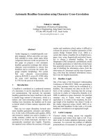
average number of words per story is 297. The
news programs are further divided chronologi-
cally into training (for parameter estimation of
the statistical models), development (for tuning
decision thresholds) and test (for performance
evaluation) sets, as shown in Figure 1. Automatic
speech recognition (ASR) outputs that are pro-
vided in the TDT-2 corpus are used for lexical
chain formation.

265
The story segmentation task in this work is to
decide whether a hypothesized utterance boun-
dary (provided in the TDT-2 data based on the
speech recognition result) is a story boundary.
Segmentation performance is evaluated using the
F1-measure.
20
hour
10
hour
10
hour
Feb.20th,1998 Mar.4th,1998 Mar.17th,1998 Apr.4th,1998
Training Set Development Set Test Set
697 stories 385 stories 376 stories
20
hour
10
hour
10
hour
Feb.20th,1998 Mar.4th,1998 Mar.17th,1998 Apr.4th,1998
Training Set Development Set Test Set
697 stories 385 stories 376 stories

Figure 1: Organization of the long programs in TDT-2
VOA Mandarin for our experiments.
3 Approach
Our approach considers utterance boundaries that

are labeled in the TDT-2 corpus and classifies
them either as a story boundary or non-boundary.
We form lexical chains from the TDT-2 ASR
outputs by linking repeated words. Since words
may also repeat across different stories, we limit
the maximum distance between consecutive
words within the lexical chain. This limit is op-
timized according to the approach in (Chan et al.
2007) based on the training data. The optimal
value is found to be 130.9sec for long programs.
We make use of three lexical chain features:
chain starts, continuations and ends. At the be-
ginning of a story, new words are introduced
more frequently and hence we observe many lex-
ical chain starts. There is also tendency of many
lexical chains ending before a story ends. As a
result, there is a higher density of chain starts and
ends in the proximity of a story boundary. Fur-
thermore, there tends to be fewer chains strad-
dling across a story boundary. Based on these
characteristics of lexical chains, we devise a sta-
tistical framework for story segmentation by
modeling the distribution of these lexical chain
features near the story boundaries.
3.1 Story Segmentation based on a Single
Lexical Chain Feature
Given an utterance boundary with the lexical
chain feature, X, we compare the conditional
probabilities of observing a boundary, B, or non-
boundary,

B
, as

<
>
)|()|( X
B
PXB
P
<
>
)|()|( X
B
PXB
P
. (1)
where X is a single chain feature, which may be
the chain start (S), chain continuation (C), or
chain end (E).
By applying the Bayes’ theorem, this can be
rewritten as a likelihood ratio test,

B
x
XP
BXP
θ
)|(
)|(
<

>
B
x
XP
BXP
θ
)|(
)|(
<
>

(2)
for which the decision threshold
is
)(/)( BPBP
x
=
θ
, dependent on the a priori
probability of observing boundary or a non-
boundary.
3.2 Story Segmentation based on Combined
Chain Features
When multiple features are used in combination,
we formulate the problem as

),,|(),,|( CESBPCESB
P
<
>

),,|(),,|( CESBPCESB
P
<
>
. (3)

By assuming that the chain features are condi-
tionally independent of one another (i.e.,
P(S,C,E|B) = P(S|B) P(C|B) P(E|B)), the formu-
lation can be rewritten as a likelihood ratio test

<
>
SEC
BCPBEPBSP
BCPBEPBSP
θ
)|()|()|(
)|()|()|(
<
>
SEC
BCPBEPBSP
BCPBEPBSP
θ
)|()|()|(
)|()|()|(
.

(4)

4 Modeling of Lexical Chain Features
4.1 Chain starts and ends
We follow (Chan et al. 2007) to model the lexi-
cal chain starts and ends at a story boundary with
a statistical distribution. We apply a window
around the candidate boundaries (same window
size for both chain starts and ends) in our work.
Chain features falling outside the window are
excluded from the model. Figure 2 shows the
distribution when a window size of 20 seconds is
used. This is the optimal window size when
chain start and end features are combined.
0
-2-4-6-8-10-12-14-16-18-20
2 4 6 8 10 12 14 16 18 20
10
20
30
40
50
Offset from story boundary in second
Number of lexical chain features
Fitted Weibull dist. for
lexical chain ends
Frequency of lexical
chain features
Fitted Weibull dist. for
lexical chain starts
x
0

-2-4-6-8-10-12-14-16-18-20
2 4 6 8 10 12 14 16 18 20
10
20
30
40
50
Offset from story boundary in second
Number of lexical chain features
Fitted Weibull dist. for
lexical chain ends
Frequency of lexical
chain features
Fitted Weibull dist. for
lexical chain starts
x
Fitted Weibull dist. for
lexical chain ends
Frequency of lexical
chain features
Fitted Weibull dist. for
lexical chain starts
x

Figure 2: Distribution of chain starts and ends at
known story boundaries. The Weibull distribution is
used to model these distributions.
We also assume that the probability of seeing
a lexical chain start / end at a particular instance
is independent of the starts / ends of other chains.

As a result, the probability of seeing a sequence
of chain starts at a story boundary is given by the
product of a sequence of Weibull distributions

∏
=






−
−






=
s
k
i
N
i
t
k
i
e

tk
BSP
1
1
)|(
λ
λλ
, (5)
266
where S is the sequence of time with chain starts
(S=[t
1
, t
2
, … t
i
, … t
Ns
]), k
s
is the shape,
λ
s
is the
scale for the fitted Weibull distribution for chain
starts, N
s
is the number of chain starts. The same
formulation is similarly applied to chain ends.
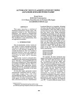
Figure 3 shows the frequency of raw feature

points for lexical chain starts and ends near utter-
ance boundaries that are non-story boundaries.
Since there is no obvious distribution pattern for
these lexical chain features near a non-story
boundary, we model these characteristics with a
uniform distribution.

2 4 6 8 10 12 14 16
0.02
0.04
0.06
0.08
0
-2-4-6-8-10-12-14-16
0.1
Relative frequency of chain starts / ends
Offset from utterance boundary in seconds
(non-story boundaries only)
Lexical chain starts / ends
Fitted uniform dist. for
lexical chain starts
x
Fitted uniform dist. for
lexical chain ends
2 4 6 8 10 12 14 16
0.02
0.04
0.06
0.08
0

-2-4-6-8-10-12-14-16
0.1
Relative frequency of chain starts / ends
Offset from utterance boundary in seconds
(non-story boundaries only)
Lexical chain starts / ends
Fitted uniform dist. for
lexical chain starts
x
Fitted uniform dist. for
lexical chain ends
Lexical chain starts / ends
Fitted uniform dist. for
lexical chain starts
x
Fitted uniform dist. for
lexical chain ends

Figure 3: Distribution of chain starts and ends at ut-
terance boundaries that are non-story boundaries.
4.2 Chain continuations
Figure 4 shows the distributions of chain contin-
uations near story boundary and non-story boun-
dary. As one may expect, there are fewer lexical
chains that straddle across a story boundary (the
curve of
)|( BCP
) when compared to a non-story
boundary (the curve of
)|( BCP

). Based on the
observations, we model the probability of occur-
rence of lexical chains straddling across a given
story boundary or non-story boundary by a nor-
mal distribution.
0
0.02
0.04
0.06
0.08
0.1
0.12
0.14
0.16
Probability
0 5 10 15 20 25
Number of chain continuations straddling across an
utterance boundary
Story
boundary,
)|( BCP
Non-story
boundary,
)|( BCP
Relative frequency of lexical chain
continuation at an utterance boundary
x
Fitted distribution at story boundary
Fitted distribution at non-story boundary
0

0.02
0.04
0.06
0.08
0.1
0.12
0.14
0.16
Probability
0 5 10 15 20 25
Number of chain continuations straddling across an
utterance boundary
Story
boundary,
)|( BCP
Non-story
boundary,
)|( BCP
Relative frequency of lexical chain
continuation at an utterance boundary
x
Fitted distribution at story boundary
Fitted distribution at non-story boundary
Relative frequency of lexical chain
continuation at an utterance boundary
x
Fitted distribution at story boundary
Fitted distribution at non-story boundary

Figure 4: Distributions of chain continuations at story

boundaries and non-story boundaries.
5 Story Segmentation based on Combi-
nation of Lexical Chain Features
We trained the parameters of the Weibull distri-
bution for lexical chain starts and ends at story
boundaries, the uniform distribution for lexical
chain start / end at non-story boundary, and the
normal distribution for lexical chain continua-
tions. Instead of directly using a threshold as
shown in Equation (2), we optimize on the para-
meter n, which is the optimal number of top scor-
ing utterance boundaries that are classified as
story boundaries in the development set.
5.1 Using Bayesian decision framework
We compare the performance of the Bayesian
decision framework to the use of likelihood only
P(X|B) as shown in Figure 5. The results demon-
strate consistent improvement in F1-measure
when using the Bayesian decision framework.
0
0.2
0.4
0.6
F1- measure
)|( BSP )|( BEP
)|(
)|(
B
SP
BSP

)|(
)|(
BEP
BEP
0
0.2
0.4
0.6
F1- measure
)|( BSP )|( BSP )|( BEP )|( BEP
)|(
)|(
B
SP
BSP
)|(
)|(
B
SP
BSP
)|(
)|(
BEP
BEP
)|(
)|(
BEP
BEP

Figure 5: Story segmentation performance in F1-

measure when using single lexical chain features.
5.2 Modeling multiple features jointly
0
0.2
0.4
0.6
0.8
F1- measure
(a) (b) (c) (d) (e) (f) (g) (h)
)|(
)|(
(c)
BEP
BEP
)|(
)|(
(d)
BCP
BCP
)|()|(
)|()|(
(e)
BEPBSP
BEPBSP
)|()|(
)|()|(
(f)
BCPBSP
BCPBSP
)|()|(

)|()|(
(g)
BCPBEP
BCPBEP
)|()|()|(
)|()|()|(
(h)
BCPBEPBSP
BCPBEPBSP
)|(
)|(
(b)
BSP
BSP
]2007[),(core (a)
Chan
E
S
S
0
0.2
0.4
0.6
0.8
F1- measure
(a) (b) (c) (d) (e) (f) (g) (h)
)|(
)|(
(c)
BEP

BEP
)|(
)|(
(d)
BCP
BCP
)|()|(
)|()|(
(e)
BEPBSP
BEPBSP
)|()|(
)|()|(
(f)
BCPBSP
BCPBSP
)|()|(
)|()|(
(g)
BCPBEP
BCPBEP
)|()|()|(
)|()|()|(
(h)
BCPBEPBSP
BCPBEPBSP
)|(
)|(
(b)
BSP

BSP
]2007[),(core (a)
Chan
E
S
S

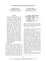
Figure 6: Results of F1-measure comparing the seg-
mentation results using different statistical models of
lexical chain features.
We further compare the performance of various
scoring methods including single and combined
lexical chain features. The baseline result is ob-
tained using a scoring function based on the like-
lihoods of seeing a chain start or end at a story
boundary (Chan et al. 2007) which is denoted as
Score(S, E). Performance from other methods
based on the same dataset can be referenced from
Chan et al. 2007 and will not be repeated here.
The best story segmentation performance is
achieved by combining all lexical chain features
which achieves an F1-measure of 0.6356. All
improvements have been verified to be statisti-
cally significant (α=0.05). By comparing the re-
sults of (e) to (h), (c) to (g), and (b) to (f), we can
see that lexical chain continuation feature contri-
butes significantly and consistently towards story
segmentation performance.
267
5.3 Analysis

Utterance boundary
(occurs at 664 second in document VOM19980317_0900_1000,
which is not a story boundary)
time
5 10-5-10
11 chain continuations:
W
1
[选出
选出选出
选出], W
2
[总理
总理总理
总理], W
3
[职务
职务职务
职务], W
4
[基本上
基本上基本上
基本上], W
5
[年代
年代年代
年代],
W
6
[就是

就是就是
就是], W
7
[中国
中国中国
中国], W
8
[中央
中央中央
中央], W
9
[主席
主席主席
主席], W
10
[都是
都是都是
都是], W
11
[国家
国家国家
国家]
15-15
W
1
5
[
人
士
人

士
人
士
人
士
]
W
1
6
[
方
面
方
面
方
面
方
面
]
W
1
7
[
委
员
会
委
员
会
委

员
会
委
员
会
]
W
1
8
[
军
事
军
事
军
事
军
事
]
W
1
9
[
连
任
连
任
连
任
连

任
]
W
2
0
[
万
年
万
年
万
年
万
年
]
W
2
1
[
浩
田
浩
田
浩
田
浩
田
]
W
1

2
[
人
选
人
选
人
选
人
选
]
W
1
3
[
最
高
最
高
最
高
最
高
]
W
1
4
[
就
说

就
说
就
说
就
说
]
t
s1
t
s2
t
s3
t
s4
t
s5
t
s6
t
s7
t
e1
t
e2
t
e3
Utterance boundary
(occurs at 664 second in document VOM19980317_0900_1000,
which is not a story boundary)

time
5 10-5-10
11 chain continuations:
W
1
[选出
选出选出
选出], W
2
[总理
总理总理
总理], W
3
[职务
职务职务
职务], W
4
[基本上
基本上基本上
基本上], W
5
[年代
年代年代
年代],
W
6
[就是
就是就是
就是], W
7

[中国
中国中国
中国], W
8
[中央
中央中央
中央], W
9
[主席
主席主席
主席], W
10
[都是
都是都是
都是], W
11
[国家
国家国家
国家]
15-15
W
1
5
[
人
士
人
士
人
士

人
士
]
W
1
6
[
方
面
方
面
方
面
方
面
]
W
1
7
[
委
员
会
委
员
会
委
员
会
委

员
会
]
W
1
8
[
军
事
军
事
军
事
军
事
]
W
1
9
[
连
任
连
任
连
任
连
任
]
W

2
0
[
万
年
万
年
万
年
万
年
]
W
2
1
[
浩
田
浩
田
浩
田
浩
田
]
W
1
2
[
人

选
人
选
人
选
人
选
]
W
1
3
[
最
高
最
高
最
高
最
高
]
W
1
4
[
就
说
就
说
就

说
就
说
]
t
s1
t
s2
t
s3
t
s4
t
s5
t
s6
t
s7
t
e1
t
e2
t
e3

Figure 7: Lexical chain starts, ends and continuations
in the proximity of a non-story boundary. W
i
[xxxx]
denotes the i-th Chinese word “xxxx”.

Figure 7 shows an utterance boundary that is a
non-story boundary. There is a high concentra-
tion of chain starts and ends near the boundary
which leads to a misclassification if we only
combine chain starts and ends for segmentation.
However, there are also a large number of chain
continuations across the utterance boundary,
which implies that a story boundary is less likely.
The full combination gives the correct decision.
Utterance boundary
(occurs at 2014 second in document
VOM19980319_0900_1000, which is a story boundary)
time
10 201020
t
s1
t
s3
t
e4
t
e5
t
e6
t
e1
t
e2
t
e3

t
s2
6 chain continuations:
W
1
[领导人
领导人领导人
领导人], W
2
[要求
要求要求
要求], W
3
[委员会
委员会委员会
委员会],
W
4
[社会
社会社会
社会], W
5
[问题
问题问题
问题, W
6
[国际
国际国际
国际]
W

1
3
[
阿
尔
巴
尼
亚
阿
尔
巴
尼
亚
阿
尔
巴
尼
亚
阿
尔
巴
尼
亚
]
W
1
4
[
塞
尔

维
亚
塞
尔
维
亚
塞
尔
维
亚
塞
尔
维
亚
]
W
1
5
[
总
统
总
统
总
统
总
统
]
W
1

2
[
成
员
成
员
成
员
成
员
]
W
1
1
[
议
会
议
会
议
会
议
会
]
W
1
0
[
柬
埔

寨
柬
埔
寨
柬
埔
寨
柬
埔
寨
]
W
9
[
时
候
时
候
时
候
时
候
]
W
8
[
大
选
大
选

大
选
大
选
]
W
7
[
宪
法
宪
法
宪
法
宪
法
]
Utterance boundary
(occurs at 2014 second in document
VOM19980319_0900_1000, which is a story boundary)
time
10 201020
t
s1
t
s3
t
e4
t
e5

t
e6
t
e1
t
e2
t
e3
t
s2
6 chain continuations:
W
1
[领导人
领导人领导人
领导人], W
2
[要求
要求要求
要求], W
3
[委员会
委员会委员会
委员会],
W
4
[社会
社会社会
社会], W
5

[问题
问题问题
问题, W
6
[国际
国际国际
国际]
W
1
3
[
阿
尔
巴
尼
亚
阿
尔
巴
尼
亚
阿
尔
巴
尼
亚
阿
尔
巴
尼

亚
]
W
1
4
[
塞
尔
维
亚
塞
尔
维
亚
塞
尔
维
亚
塞
尔
维
亚
]
W
1
5
[
总
统
总

统
总
统
总
统
]
W
1
2
[
成
员
成
员
成
员
成
员
]
W
1
1
[
议
会
议
会
议
会
议

会
]
W
1
0
[
柬
埔
寨
柬
埔
寨
柬
埔
寨
柬
埔
寨
]
W
9
[
时
候
时
候
时
候
时
候

]
W
8
[
大
选
大
选
大
选
大
选
]
W
7
[
宪
法
宪
法
宪
法
宪
法
]

Figure 8: Lexical chain starts, ends and continuations
in the proximity of a story boundary.
Figure 8 shows another example where an ut-
terance boundary is misclassified as a non-story

boundary when only the combination of lexical
chain starts and ends are used. Incorporation of
the chain continuation feature helps rectify the
classification.
From these two examples, we can see that the
incorporation of chain continuation in our story
segmentation framework can complement the
features of chain starts and ends. In both exam-
ples above, the number of chain continuations
plays a crucial role in correct identification of a
story boundary.
6 Conclusions
We have presented a Bayesian decision frame-
work that performs automatic story segmentation
based on statistical modeling of one or more lex-
ical chain features, including lexical chain starts,
continuations and ends. Experimentation shows
that the Bayesian decision framework is superior
to the use of likelihoods for segmentation. We
also experimented with a variety of scoring crite-
ria, involving likelihood ratio tests of a single
feature (i.e. lexical chain starts, continuations or
ends), their pair-wise combinations, as well as
the full combination of all three features. Lexical
chain starts/ends are modeled statistically with
the Weibull and normal distributions for story
boundaries and non-boundaries. The normal dis-
tribution is used for lexical chain continuations.
Full combination of all lexical chain features
gave the best performance (F1=0.6356). Model-

ing chain continuations contribute significantly
towards segmentation performance.
Acknowledgments
This work is affiliated with the CUHK MoE-
Microsoft Key Laboratory of Human-centric Compu-
ting and Interface Technologies. We would also like
to thank Professor Mari Ostendorf for suggesting the
use of continuing chains and Mr. Kelvin Chan for
providing information about his previous work.

References
Chan, S. K. et al. 2007. “Modeling the Statistical Be-
haviour of Lexical Chains to Capture Word Cohe-
siveness for Automatic Story Segmentation”, Proc.
of INTERSPEECH-2007.
Hearst, M. A. 1997. “TextTiling: Segmenting Text
into Multiparagraph Subtopic Passages”, Computa-
tional Linguistics, 23(1), pp. 33–64.
Hirst, G. and St-Onge, D. 1998. “Lexical chains as
representations of context for the detection and
correction of malapropisms”, WordNet: An Elec-
tronic Lexical Database, pp. 305–332.
Morris, J. and Hirst, G. 1991. “Lexical cohesion com-
puted by thesaural relations as an indicator of the
structure of text”, Computational Linguistics,
17(1), pp. 21–48.
Reynar, J.C. 1999, “Statistical models for topic seg-
mentation”, Proc. 37th annual meeting of the ACL,
pp. 357–364.
Stokes, N. 2004. Applications of Lexical Cohesion

Analysis in the Topic Detection and Tracking Do-
main, PhD thesis, University College Dublin.
Yamron, J.P. et al. 1998, “A hidden Markov model
approach to text segmentation and event tracking”,
Proc. ICASSP 1998, pp. 333–336.
268