Báo cáo khoa học: "Guessing Parts-of-Speech of Unknown Words Using Global Information" ppt
Bạn đang xem bản rút gọn của tài liệu. Xem và tải ngay bản đầy đủ của tài liệu tại đây (539.19 KB, 8 trang )
Proceedings of the 21st International Conference on Computational Linguistics and 44th Annual Meeting of the ACL, pages 705–712,
Sydney, July 2006.
c
2006 Association for Computational Linguistics
Guessing Parts-of-Speech of Unknown Words Using Global Information
Tetsuji Nakagawa
Corporate R&D Center
Oki Electric Industry Co., Ltd.
2−5−7 Honmachi, Chuo-ku
Osaka 541−0053, Japan
Yuji Matsumoto
Graduate School of Information Science
Nara Institute of Science and Technology
8916−5 Takayama, Ikoma
Nara 630−0101, Japan
Abstract
In this paper, we present a method for
guessing POS tags of unknown words us-
ing local and global information. Al-
though many existing methods use only
local information (i.e. limited window
size or intra-sentential features), global in-
formation (extra-sentential features) pro-
vides valuable clues for predicting POS
tags of unknown words. We propose a
probabilistic model for POS guessing of
unknown words using global information
as well as local information, and estimate
its parameters using Gibbs sampling. We
also attempt to apply the model to semi-
supervised learning, and conduct experi-
ments on multiple corpora.
1 Introduction
Part-of-speech (POS) tagging is a fundamental
language analysis task. In POS tagging, we fre-
quently encounter words that do not exist in train-
ing data. Such words are called unknown words.
They are usually handled by an exceptional pro-
cess in POS tagging, because the tagging sys-
tem does not have information about the words.
Guessing the POS tags of such unknown words is
a difficult task. But it is an important issue both
for conducting POS tagging accurately and for
creating word dictionaries automatically or semi-
automatically. There have been many studies on
POS guessing of unknown words (Mori and Na-
gao, 1996; Mikheev, 1997; Chen et al., 1997; Na-
gata, 1999; Orphanos and Christodoulakis, 1999).
In most of these previous works, POS tags of un-
known words were predicted using only local in-
formation, such as lexical forms and POS tags
of surrounding words or word-internal features
(e.g. suffixes and character types) of the unknown
words. However, this approach has limitations
in available information. For example, common
nouns and proper nouns are sometimes difficult
to distinguish with only the information of a sin-
gle occurrence because their syntactic functions
are almost identical. In English, proper nouns
are capitalized and there is generally little ambi-
guity between common nouns and proper nouns.
In Chinese and Japanese, no such convention ex-
ists and the problem of the ambiguity is serious.
However, if an unknown word with the same lex-
ical form appears in another part with informa-
tive local features (e.g. titles of persons), this will
give useful clues for guessing the part-of-speech
of the ambiguous one, because unknown words
with the same lexical form usually have the same
part-of-speech. For another example, there is a
part-of-speech named sahen-noun (verbal noun) in
Japanese. Verbal nouns behave as common nouns,
except that they are used as verbs when they are
followed by a verb “suru”; e.g., a verbal noun
“dokusho” means “reading” and “dokusho-suru”
is a verb meaning to “read books”. It is diffi-
cult to distinguish a verbal noun from a common
noun if it is used as a noun. However, it will
be easy if we know that the word is followed by
“suru” in another part in the document. This issue
was mentioned by Asahara (2003) as a problem
of possibility-based POS tags. A possibility-based
POS tag is a POS tag that represents all the possi-
ble properties of the word (e.g., a verbal noun is
used as a noun or a verb), rather than a property of
each instance of the word. For example, a sahen-
noun is actually a noun that can be used as a verb
when it is followed by “suru”. This property can-
not be confirmed without observing real usage of
the word appearing with “suru”. Such POS tags
may not be identified with only local information
of one instance, because the property that each in-
stance has is only one among all the possible prop-
erties.
To cope with these issues, we propose a method
that uses global information as well as local in-
formation for guessing the parts-of-speech of un-
known words. With this method, all the occur-
rences of the unknown words in a document
1
are
taken into consideration at once, rather than that
each occurrence of the words is processed sepa-
rately. Thus, the method models the whole doc-
ument and finds a set of parts-of-speech by max-
imizing its conditional joint probability given the
document, rather than independently maximizing
the probability of each part-of-speech given each
sentence. Global information is known to be use-
ful in other NLP tasks, especially in the named en-
tity recognition task, and several studies success-
fully used global features (Chieu and Ng, 2002;
Finkel et al., 2005).
One potential advantage of our method is its
1
In this paper, we use the word document to denote the
whole data consisting of multiple sentences (training corpus
or test corpus).
705
ability to incorporate unlabeled data. Global fea-
tures can be increased by simply adding unlabeled
data into the test data.
Models in which the whole document is taken
into consideration need a lot of computation com-
pared to models with only local features. They
also cannot process input data one-by-one. In-
stead, the entire document has to be read before
processing. We adopt Gibbs sampling in order to
compute the models efficiently, and these models
are suitable for offline use such as creating dictio-
naries from raw text where real-time processing is
not necessary but high-accuracy is needed to re-
duce human labor required for revising automati-
cally analyzed data.
The rest of this paper is organized as follows:
Section 2 describes a method for POS guessing of
unknown words which utilizes global information.
Section 3 shows experimental results on multiple
corpora. Section 4 discusses related work, and
Section 5 gives conclusions.
2 POS Guessing of Unknown Words with
Global Information
We handle POS guessing of unknown words as a
sub-task of POS tagging, in this paper. We assume
that POS tags of known words are already deter-
mined beforehand, and positions in the document
where unknown words appear are also identified.
Thus, we focus only on prediction of the POS tags
of unknown words.
In the rest of this section, we first present a
model for POS guessing of unknown words with
global information. Next, we show how the test
data is analyzed and how the parameters of the
model are estimated. A method for incorporating
unlabeled data with the model is also discussed.
2.1 Probabilistic Model Using Global
Information
We attempt to model the probability distribution
of the parts-of-speech of all occurrences of the
unknown words in a document which have the
same lexical form. We suppose that such parts-
of-speech have correlation, and the part-of-speech
of each occurrence is also affected by its local
context. Similar situations to this are handled in
physics. For example, let us consider a case where
a number of electrons with spins exist in a system.
The spins interact with each other, and each spin is
also affected by the external magnetic field. In the
physical model, if the state of the system is s and
the energy of the system is E(s), the probability
distribution of s is known to be represented by the
following Boltzmann distribution:
P (s)=
1
Z
exp{−βE(s)}, (1)
where β is inverse temperature and Z is a normal-
izing constant defined as follows:
Z=
s
exp{−βE(s)}. (2)
Takamura et al. (2005) applied this model to an
NLP task, semantic orientation extraction, and we
apply it to POS guessing of unknown words here.
Suppose that unknown words with the same lex-
ical form appear K times in a document. Assume
that the number of possible POS tags for unknown
words is N, and they are represented by integers
from 1 to N . Let t
k
denote the POS tag of the kth
occurrence of the unknown words, let w
k
denote
the local context (e.g. the lexical forms and the
POS tags of the surrounding words) of the kth oc-
currence of the unknown words, and let w and t
denote the sets of w
k
and t
k
respectively:
w ={w
1
, ···, w
K
}, t={t
1
, ···, t
K
}, t
k
∈{1, ···, N}.
λ
i,j
is a weight which denotes strength of the in-
teraction between parts-of-speech i and j, and is
symmetric (λ
i,j
= λ
j,i
). We define the energy
where POS tags of unknown words given w are
t as follows:
E(t|w)=−
1
2
K
k=1
K
k
=1
k
=k
λ
t
k
,t
k
+
K
k=1
log p
0
(t
k
|w
k
)
,
(3)
where p
0
(t|w) is an initial distribution (local
model) of the part-of-speech t which is calculated
with only the local context w , using arbitrary sta-
tistical models such as maximum entropy models.
The right hand side of the above equation consists
of two components; one represents global interac-
tions between each pair of parts-of-speech, and the
other represents the effects of local information.
In this study, we fix the inverse temperature
β = 1. The distribution of t is then obtained from
Equation (1), (2) and (3) as follows:
P (t|w)=
1
Z(w)
p
0
(t|w) exp
1
2
K
k=1
K
k
=1
k
=k
λ
t
k
,t
k
, (4)
Z(w)=
t∈T (w)
p
0
(t|w) exp
1
2
K
k=1
K
k
=1
k
=k
λ
t
k
,t
k
, (5)
p
0
(t|w)≡
K
k=1
p
0
(t
k
|w
k
), (6)
where T (w) is the set of possible configurations
of POS tags given w. The size of T (w) is N
K
,
because there are K occurrences of the unknown
words and each unknown word can have one of N
POS tags. The above equations can be rewritten as
follows by defining a function f
i,j
(t):
f
i,j
(t)≡
1
2
K
k=1
K
k
=1
k
=k
δ(t
k
, i ) δ(t
k
, j), (7)
P (t|w)=
1
Z(w)
p
0
(t|w) exp
N
i=1
N
j=1
λ
i,j
f
i,j
(t)
, (8)
Z(w)=
t∈T (w)
p
0
(t|w) exp
N
i=1
N
j=1
λ
i,j
f
i,j
(t)
, (9)
706
where δ(i, j) is the Kronecker delta:
δ(i, j)=
1 (i = j),
0 (i = j).
(10)
f
i,j
(t) represents the number of occurrences of the
POS tag pair i and j in the whole document (di-
vided by 2), and the model in Equation (8) is es-
sentially a maximum entropy model with the doc-
ument level features.
As shown above, we consider the conditional
joint probability of all the occurrences of the un-
known words with the same lexical form in the
document given their local contexts, P (t|w ), in
contrast to conventional approaches which assume
independence of the sentences in the document
and use the probabilities of all the words only in
a sentence. Note that we assume independence
between the unknown words with different lexical
forms, and each set of the unknown words with the
same lexical form is processed separately from the
sets of other unknown words.
2.2 Decoding
Let us consider how to find the optimal POS tags t
basing on the model, given K local contexts of the
unknown words with the same lexical form (test
data) w, an initial distribution p
0
(t|w) and a set
of model parameters Λ = {λ
1,1
, ···, λ
N,N
}. One
way to do this is to find a set of POS tags which
maximizes P (t|w) among all possible candidates
of t. However, the number of all possible candi-
dates of the POS tags is N
K
and the calculation is
generally intractable. Although HMMs, MEMMs,
and CRFs use dynamic programming and some
studies with probabilistic models which have spe-
cific structures use efficient algorithms (Wang et
al., 2005), such methods cannot be applied here
because we are considering interactions (depen-
dencies) between all POS tags, and their joint dis-
tribution cannot be decomposed. Therefore, we
use a sampling technique and approximate the so-
lution using samples obtained from the probability
distribution.
We can obtain a solution
ˆ
t = {
ˆ
t
1
, ···,
ˆ
t
K
} as
follows:
ˆ
t
k
=argmax
t
P
k
(t|w), (11)
where P
k
(t|w) is the marginal distribution of the
part-of-speech of the kth occurrence of the un-
known words given a set of local contexts w, and
is calculated as an expected value over the distri-
bution of the unknown words as follows:
P
k
(t|w)=
t
1
,···,t
k−1
,t
k+1
,···,t
K
t
k
=t
P (t|w),
=
t∈T (w)
δ(t
k
, t)P (t|w). (12)
Expected values can be approximately calculated
using enough number of samples generated from
the distribution (MacKay, 2003). Suppose that
A(x) is a function of a random variable x, P(x)
initialize t
(1)
for m := 2 to M
for k := 1 to K
t
(m)
k
∼ P (t
k
|w, t
(m)
1
, ···, t
(m)
k−1
, t
(m−1)
k+1
, ···, t
(m−1)
K
)
Figure 1: Gibbs Sampling
is a distribution of x, and {x
(1)
, ···, x
(M)
} are M
samples generated from P(x). Then, the expec-
tation of A(x) over P (x) is approximated by the
samples:
x
A(x)P (x)
1
M
M
m=1
A(x
(m)
). (13)
Thus, if we have M samples {t
(1)
, ···, t
(M)
}
generated from the conditional joint distribution
P (t|w), the marginal distribution of each POS tag
is approximated as follows:
P
k
(t|w)
1
M
M
m=1
δ(t
(m)
k
, t ). (14)
Next, we describe how to generate samples
from the distribution. We use Gibbs sampling
for this purpose. Gibbs sampling is one of the
Markov chain Monte Carlo (MCMC) methods,
which can generate samples efficiently from high-
dimensional probability distributions (Andrieu et
al., 2003). The algorithm is shown in Figure 1.
The algorithm firstly set the initial state t
(1)
, then
one new random variable is sampled at a time
from the conditional distribution in which all other
variables are fixed, and new samples are cre-
ated by repeating the process. Gibbs sampling is
easy to implement and is guaranteed to converge
to the true distribution. The conditional distri-
bution P (t
k
|w, t
1
, ···, t
k−1
, t
k+1
, ···, t
K
) in Fig-
ure 1 can be calculated simply as follows:
P (t
k
|w, t
1
, ···, t
k−1
, t
k+1
, ···, t
K
)
=
P (t|w)
P (t
1
, ···, t
k−1
, t
k+1
, ···, t
K
|w)
,
=
1
Z(w)
p
0
(t|w) exp{
1
2
K
k
=1
K
k
=1
k
=k
λ
t
k
,t
k
}
N
t
∗
k
=1
P (t
1
, ···, t
k−1
, t
∗
k
, t
k+1
, ···, t
K
|w)
,
=
p
0
(t
k
|w
k
) exp{
K
k
=1
k
=k
λ
t
k
,t
k
}
N
t
∗
k
=1
p
0
(t
∗
k
|w
k
) exp {
K
k
=1
k
=k
λ
t
k
,t
∗
k
}
, (15)
where the last equation is obtained using the fol-
lowing relation:
1
2
K
k
=1
K
k
=1
k
=k
λ
t
k
,t
k
=
1
2
K
k
=1
k
=k
K
k
=1
k
=k,k
=k
λ
t
k
,t
k
+
K
k
=1
k
=k
λ
t
k
,t
k
.
In later experiments, the number of samples M is
set to 100, and the initial state t
(1)
is set to the POS
tags which maximize p
0
(t|w).
The optimal solution obtained by Equation (11)
maximizes the probability of each POS tag given
w, and this kind of approach is known as the maxi-
mum posterior marginal (MPM) estimate (Marro-
quin, 1985). Finkel et al. (2005) used simulated
annealing with Gibbs sampling to find a solution
in a similar situation. Unlike simulated annealing,
this approach does not need to define a cooling
707
schedule. Furthermore, this approach can obtain
not only the best solution but also the second best
or the other solutions according to P
k
(t|w), which
are useful when this method is applied to semi-
automatic construction of dictionaries because hu-
man annotators can check the ranked lists of can-
didates.
2.3 Parameter Estimation
Let us consider how to estimate the param-
eter Λ = {λ
1,1
, ···, λ
N,N
} in Equation (8)
from training data consisting of L examples;
{w
1
, t
1
, ···, w
L
, t
L
} (i.e., the training data
contains L different lexical forms of unknown
words). We define the following objective func-
tion L
Λ
, and find Λ which maximizes L
Λ
(the sub-
script Λ denotes being parameterized by Λ):
L
Λ
= log
L
l=1
P
Λ
(t
l
|w
l
) + log P (Λ),
= log
L
l=1
1
Z
Λ
(w
l
)
p
0
(t
l
|w
l
) exp
N
i=1
N
j=1
λ
i,j
f
i,j
(t
l
)
+ log P (Λ),
=
L
l=1
−log Z
Λ
(w
l
)+log p
0
(t
l
|w
l
)+
N
i=1
N
j=1
λ
i,j
f
i,j
(t
l
)
+ log P (Λ). (16)
The partial derivatives of the objective function
are:
∂L
Λ
∂λ
i,j
=
L
l=1
f
i,j
(t
l
)−
∂
∂λ
i,j
log Z
Λ
(w
l
)
+
∂
∂λ
i,j
log P(Λ),
=
L
l=1
f
i,j
(t
l
) −
t∈T (w
l
)
f
i,j
(t)P
Λ
(t|w
l
)
+
∂
∂λ
i,j
log P(Λ).
(17)
We use Gaussian priors (Chen and Rosenfeld,
1999) for P (Λ):
log P(Λ)=−
N
i=1
N
j=1
λ
2
i,j
2σ
2
+ C,
∂
∂λ
i,j
log P(Λ) = −
λ
i,j
σ
2
.
where C is a constant and σ is set to 1 in later
experiments. The optimal Λ can be obtained by
quasi-Newton methods using the above L
Λ
and
∂L
Λ
∂λ
i,j
, and we use L-BFGS (Liu and Nocedal,
1989) for this purpose
2
. However, the calculation
is intractable because Z
Λ
(w
l
) (see Equation (9))
in Equation (16) and a term in Equation (17) con-
tain summations over all the possible POS tags. To
cope with the problem, we use the sampling tech-
nique again for the calculation, as suggested by
Rosenfeld et al. (2001). Z
Λ
(w
l
) can be approx-
imated using M samples {t
(1)
, ···, t
(M)
} gener-
ated from p
0
(t|w
l
):
Z
Λ
(w
l
)=
t∈T (w
l
)
p
0
(t|w
l
) exp
N
i=1
N
j=1
λ
i,j
f
i,j
(t)
,
2
In later experiments, L-BFGS often did not converge
completely because we used approximation with Gibbs sam-
pling, and we stopped iteration of L-BFGS in such cases.
1
M
M
m=1
exp
N
i=1
N
j=1
λ
i,j
f
i,j
(t
(m)
)
. (18)
The term in Equation (17) can also be approxi-
mated using M samples {t
(1)
, ···, t
(M)
} gener-
ated from P
Λ
(t|w
l
) with Gibbs sampling:
t∈T (w
l
)
f
i,j
(t)P
Λ
(t|w
l
)
1
M
M
m=1
f
i,j
(t
(m)
). (19)
In later experiments, the initial state t
(1)
in Gibbs
sampling is set to the gold standard tags in the
training data.
2.4 Use of Unlabeled Data
In our model, unlabeled data can be easily used
by simply concatenating the test data and the unla-
beled data, and decoding them in the testing phase.
Intuitively, if we increase the amount of the test
data, test examples with informative local features
may increase. The POS tags of such examples can
be easily predicted, and they are used as global
features in prediction of other examples. Thus,
this method uses unlabeled data in only the test-
ing phase, and the training phase is the same as
the case with no unlabeled data.
3 Experiments
3.1 Data and Procedure
We use eight corpora for our experiments; the
Penn Chinese Treebank corpus 2.0 (CTB), a part
of the PFR corpus (PFR), the EDR corpus (EDR),
the Kyoto University corpus version 2 (KUC), the
RWCP corpus (RWC), the GENIA corpus 3.02p
(GEN), the SUSANNE corpus (SUS) and the Penn
Treebank WSJ corpus (WSJ), (cf. Table 1). All
the corpora are POS tagged corpora in Chinese(C),
English(E) or Japanese(J), and they are split into
three portions; training data, test data and unla-
beled data. The unlabeled data is used in ex-
periments of semi-supervised learning, and POS
tags of unknown words in the unlabeled data are
eliminated. Table 1 summarizes detailed informa-
tion about the corpora we used: the language, the
number of POS tags, the number of open class
tags (POS tags that unknown words can have, de-
scribed later), the sizes of training, test and un-
labeled data, and the splitting method of them.
For the test data and the unlabeled data, unknown
words are defined as words that do not appear in
the training data. The number of unknown words
in the test data of each corpus is shown in Ta-
ble 1, parentheses. Accuracy of POS guessing of
unknown words is calculated based on how many
words among them are correctly POS-guessed.
Figure 2 shows the procedure of the experi-
ments. We split the training data into two parts;
the first half as sub-training data 1 and the latter
half as sub-training data 2 (Figure 2, *1). Then,
we check the words that appear in the sub-training
708
Corpus # of POS # of Tokens (# of Unknown Words) [partition in the corpus]
(Lang.) (Open Class) Training Test Unlabeled
CTB 34 84,937 7,980 (749) 6,801
(C) (28) [sec. 1–270] [sec. 271–300] [sec. 301–325]
PFR 42 304,125 370,627 (27,774) 445,969
(C) (39) [Jan. 1–Jan. 9] [Jan. 10–Jan. 19] [Jan. 20–Jan. 31]
EDR 15 2,550,532 1,280,057 (24,178) 1,274,458
(J) (15) [id = 4n + 0, id = 4n + 1] [id = 4n + 2] [id = 4n + 3]
KUC 40 198,514 31,302 (2,477) 41,227
(J) (36) [Jan. 1–Jan. 8] [Jan. 9] [Jan. 10]
RWC 66 487,333 190,571 (11,177) 210,096
(J) (55) [1–10,000th sentences] [10,001–14,000th sentences] [14,001–18,672th sentences]
GEN 47 243,180 123,386 (7,775) 134,380
(E) (36) [1–10,000th sentences] [10,001–15,000th sentences] [15,001–20,546th sentences]
SUS 125 74,902 37,931 (5,760) 37,593
(E) (90) [sec. A01–08, G01–08, [sec. A09–12, G09–12, [sec. A13–20, G13–22,
J01–08, N01–08] J09–17, N09–12] J21–24, N13–18]
WSJ 45 912,344 129,654 (4,253) 131,768
(E) (33) [sec. 0–18] [sec. 22–24] [sec. 19–21]
Table 1: Statistical Information of Corpora
Corpus
Training
Data
Test
Data
Unlabeled
Data
Sub-
Training
data 1
(*1)
Sub-
Training
data 2
(*1)
Sub-Local Model 1
(*3)
Sub-Local Model 2
(*3)
Global Model
Local Model
(*2)
(optional)
Test
Result
Data flow for training
Data flow for testing
Figure 2: Experimental Procedure
data 1 but not in the sub-training data 2, or vice
versa. We handle these words as (pseudo) un-
known words in the training data. Such (two-fold)
cross-validation is necessary to make training ex-
amples that contain unknown words
3
. POS tags
that these pseudo unknown words have are defined
as open class tags, and only the open class tags
are considered as candidate POS tags for unknown
words in the test data (i.e., N is equal to the num-
ber of the open class tags). In the training phase,
we need to estimate two types of parameters; local
model (parameters), which is necessary to calcu-
late p
0
(t|w), and global model (parameters), i.e.,
λ
i,j
. The local model parameters are estimated
using all the training data (Figure 2, *2). Local
3
A major method for generating such pseudo unknown
words is to collect the words that appear only once in a cor-
pus (Nagata, 1999). These words are called hapax legom-
ena and known to have similar characteristics to real un-
known words (Baayen and Sproat, 1996). These words are
interpreted as being collected by the leave-one-out technique
(which is a special case of cross-validation) as follows: One
word is picked from the corpus and the rest of the corpus
is considered as training data. The picked word is regarded
as an unknown word if it does not exist in the training data.
This procedure is iterated for all the words in the corpus.
However, this approach is not applicable to our experiments
because those words that appear only once in the corpus do
not have global information and are useless for learning the
global model, so we use the two-fold cross validation method.
model parameters and training data are necessary
to estimate the global model parameters, but the
global model parameters cannot be estimated from
the same training data from which the local model
parameters are estimated. In order to estimate the
global model parameters, we firstly train sub-local
models 1 and 2 from the sub-training data 1 and
2 respectively (Figure 2, *3). The sub-local mod-
els 1 and 2 are used for calculating p
0
(t|w) of un-
known words in the sub-training data 2 and 1 re-
spectively, when the global model parameters are
estimated from the entire training data. In the test-
ing phase, p
0
(t|w) of unknown words in the test
data are calculated using the local model param-
eters which are estimated from the entire training
data, and test results are obtained using the global
model with the local model.
Global information cannot be used for unknown
words whose lexical forms appear only once in
the training or test data, so we process only non-
unique unknown words (unknown words whose
lexical forms appear more than once) using the
proposed model. In the testing phase, POS tags of
unique unknown words are determined using only
the local information, by choosing POS tags which
maximize p
0
(t|w).
Unlabeled data can be optionally used for semi-
supervised learning. In that case, the test data and
the unlabeled data are concatenated, and the best
POS tags which maximize the probability of the
mixed data are searched.
3.2 Initial Distribution
In our method, the initial distribution p
0
(t|w) is
used for calculating the probability of t given lo-
cal context w (Equation (8)). We use maximum
entropy (ME) models for the initial distribution.
p
0
(t|w) is calculated by ME models as follows
(Berger et al., 1996):
p
0
(t|w)=
1
Y (w)
exp
H
h=1
α
h
g
h
(w, t)
, (20)
709
Language Features
English Prefixes of ω
0
up to four characters,
suffixes of ω
0
up to four characters,
ω
0
contains Arabic numerals,
ω
0
contains uppercase characters,
ω
0
contains hyphens.
Chinese Prefixes of ω
0
up to two characters,
Japanese suffixes of ω
0
up to two characters,
ψ
1
, ψ
|ω
0
|
, ψ
1
& ψ
|ω
0
|
,
|ω
0
|
i=1
{ψ
i
} (set of character types).
(common) |ω
0
| (length of ω
0
),
τ
−1
, τ
+1
, τ
−2
& τ
−1
, τ
+1
& τ
+2
,
τ
−1
& τ
+1
, ω
−1
& τ
−1
, ω
+1
& τ
+1
,
ω
−2
& τ
−2
& ω
−1
& τ
−1
,
ω
+1
& τ
+1
& ω
+2
& τ
+2
,
ω
−1
& τ
−1
& ω
+1
& τ
+1
.
Table 2: Features Used for Initial Distribution
Y (w)=
N
t=1
exp
H
h=1
α
h
g
h
(w, t)
, (21)
where g
h
(w, t) is a binary feature function. We
assume that each local context w contains the fol-
lowing information about the unknown word:
• The POS tags of the two words on each side
of the unknown word: τ
−2
, τ
−1
, τ
+1
, τ
+2
.
4
• The lexical forms of the unknown word itself
and the two words on each side of the un-
known word: ω
−2
, ω
−1
, ω
0
, ω
+1
, ω
+2
.
• The character types of all the characters com-
posing the unknown word: ψ
1
, ···, ψ
|ω
0
|
.
We use six character types: alphabet, nu-
meral (Arabic and Chinese numerals), sym-
bol, Kanji (Chinese character), Hiragana
(Japanese script) and Katakana (Japanese
script).
A feature function g
h
(w, t) returns 1 if w and t
satisfy certain conditions, and otherwise 0; for ex-
ample:
g
123
(w, t)=
1 (ω
−1
=“President” and τ
−1
=“NNP” and t = 5),
0 (otherwise).
The features we use are shown in Table 2, which
are based on the features used by Ratnaparkhi
(1996) and Uchimoto et al. (2001).
The parameters α
h
in Equation (20) are esti-
mated using all the words in the training data
whose POS tags are the open class tags.
3.3 Experimental Results
The results are shown in Table 3. In the table, lo-
cal, local+global and local+global w/ unlabeled
indicate that the results were obtained using only
local information, local and global information,
and local and global information with the extra un-
labeled data, respectively. The results using only
local information were obtained by choosing POS
4
In both the training and the testing phases, POS tags of
known words are given from the corpora. When these sur-
rounding words contain unknown words, their POS tags are
represented by a special tag Unk.
PFR (Chinese)
+162 vn (verbal noun)
+150 ns (place name)
+86 nz (other proper noun)
+85 j (abbreviation)
+61 nr (personal name)
··· ···
−26 m (numeral)
−100 v (verb)
RWC (Japanese)
+33 noun-proper noun-person name-family name
+32 noun-proper noun-place name
+28 noun-proper noun-organization name
+17 noun-proper noun-person name-first name
+6 noun-proper noun
+4 noun-sahen noun
··· ···
−2 noun-proper noun-place name-country name
−29 noun
SUS (English)
+13 NP (proper noun)
+6 JJ (adjective)
+2 VVD (past tense form of lexical verb)
+2 NNL (locative noun)
+2 NNJ (organization noun)
··· ···
−3 NN (common noun)
−6 NNU (unit-of-measurement noun)
Table 4: Ordered List of Increased/Decreased
Number of Correctly Tagged Words
tags
ˆ
t = {
ˆ
t
1
, ···,
ˆ
t
K
} which maximize the proba-
bilities of the local model:
ˆ
t
k
=argmax
t
p
0
(t|w
k
). (22)
The table shows the accuracies, the numbers of er-
rors, the p-values of McNemar’s test against the
results using only local information, and the num-
bers of non-unique unknown words in the test
data. On an Opteron 250 processor with 8GB of
RAM, model parameter estimation and decoding
without unlabeled data for the eight corpora took
117 minutes and 39 seconds in total, respectively.
In the CTB, PFR, KUC, RWC and WSJ cor-
pora, the accuracies were improved using global
information (statistically significant at p < 0.05),
compared to the accuracies obtained using only lo-
cal information. The increases of the accuracies on
the English corpora (the GEN and SUS corpora)
were small. Table 4 shows the increased/decreased
number of correctly tagged words using global in-
formation in the PFR, RWC and SUS corpora.
In the PFR (Chinese) and RWC (Japanese) cor-
pora, many proper nouns were correctly tagged us-
ing global information. In Chinese and Japanese,
proper nouns are not capitalized, therefore proper
nouns are difficult to distinguish from common
nouns with only local information. One reason
that only the small increases were obtained with
global information in the English corpora seems to
be the low ambiguities of proper nouns. Many ver-
bal nouns in PFR and a few sahen-nouns (Japanese
verbal nouns) in RWC, which suffer from the
problem of possibility-based POS tags, were also
correctly tagged using global information. When
the unlabeled data was used, the number of non-
unique words in the test data increased. Compared
with the case without the unlabeled data, the accu-
710
Corpus Accuracy for Unknown Words (# of Errors)
(Lang.) [p-value] # of Non-unique Unknown Words
local local+global local+global w/ unlabeled
CTB 0.7423 (193) 0.7717 (171) 0.7704 (172)
(C) [0.0000] 344 [0.0001] 361
PFR 0.6499 (9723) 0.6690 (9193) 0.6785 (8930)
(C) [0.0000] 16019 [0.0000] 18861
EDR 0.9639 (874) 0.9643 (863) 0.9651 (844)
(J) [0.1775] 4903 [0.0034] 7770
KUC 0.7501 (619) 0.7634 (586) 0.7562 (604)
(J) [0.0000] 788 [0.0872] 936
RWC 0.7699 (2572) 0.7785 (2476) 0.7787 (2474)
(J) [0.0000] 5044 [0.0000] 5878
GEN 0.8836 (905) 0.8837 (904) 0.8863 (884)
(E) [1.0000] 4094 [0.0244] 4515
SUS 0.7934 (1190) 0.7957 (1177) 0.7979 (1164)
(E) [0.1878] 3210 [0.0116] 3583
WSJ 0.8345 (704) 0.8368 (694) 0.8352 (701)
(E) [0.0162] 1412 [0.7103] 1627
Table 3: Results of POS Guessing of Unknown Words
Corpus Mean±Standard Deviation
(Lang.) Marginal S.A.
CTB (C) 0.7696±0.0021 0.7682±0.0028
PFR (C) 0.6707±0.0010 0.6712±0.0014
EDR (J) 0.9644±0.0001 0.9645±0.0001
KUC (J) 0.7595±0.0031 0.7612±0.0018
RWC (J) 0.7777±0.0017 0.7772±0.0020
GEN (E) 0.8841±0.0009 0.8840±0.0007
SUS (E) 0.7997±0.0038 0.7995±0.0034
WSJ (E) 0.8366±0.0013 0.8360±0.0021
Table 5: Results of Multiple Trials and Compari-
son to Simulated Annealing
racies increased in several corpora but decreased
in the CTB, KUC and WSJ corpora.
Since our method uses Gibbs sampling in the
training and the testing phases, the results are af-
fected by the sequences of random numbers used
in the sampling. In order to investigate the influ-
ence, we conduct 10 trials with different sequences
of pseudo random numbers. We also conduct ex-
periments using simulated annealing in decoding,
as conducted by Finkel et al. (2005) for informa-
tion extraction. We increase inverse temperature β
in Equation (1) from β = 1 to β ≈ ∞ with the
linear cooling schedule. The results are shown in
Table 5. The table shows the mean values and the
standard deviations of the accuracies for the 10 tri-
als, and Marginal and S.A. mean that decoding is
conducted using Equation (11) and simulated an-
nealing respectively. The variances caused by ran-
dom numbers and the differences of the accuracies
between Marginal and S.A. are relatively small.
4 Related Work
Several studies concerning the use of global infor-
mation have been conducted, especially in named
entity recognition, which is a similar task to POS
guessing of unknown words. Chieu and Ng (2002)
conducted named entity recognition using global
features as well as local features. In their ME
model-based method, some global features were
used such as “when the word appeared first in a
position other than the beginning of sentences, the
word was capitalized or not”. These global fea-
tures are static and can be handled in the same
manner as local features, therefore Viterbi decod-
ing was used. The method is efficient but does not
handle interactions between labels.
Finkel et al. (2005) proposed a method incorpo-
rating non-local structure for information extrac-
tion. They attempted to use label consistency of
named entities, which is the property that named
entities with the same lexical form tend to have
the same label. They defined two probabilis-
tic models; a local model based on conditional
random fields and a global model based on log-
linear models. Then the final model was con-
structed by multiplying these two models, which
can be seen as unnormalized log-linear interpola-
tion (Klakow, 1998) of the two models which are
weighted equally. In their method, interactions be-
tween labels in the whole document were consid-
ered, and they used Gibbs sampling and simulated
annealing for decoding. Our model is largely sim-
ilar to their model. However, in their method, pa-
rameters of the global model were estimated using
relative frequencies of labels or were selected by
hand, while in our method, global model parame-
ters are estimated from training data so as to fit to
the data according to the objective function.
One approach for incorporating global infor-
mation in natural language processing is to uti-
lize consistency of labels, and such an approach
have been used in other tasks. Takamura et al.
(2005) proposed a method based on the spin mod-
els in physics for extracting semantic orientations
of words. In the spin models, each electron has
one of two states, up or down, and the models give
probability distribution of the states. The states
of electrons interact with each other and neighbor-
ing electrons tend to have the same spin. In their
711
method, semantic orientations (positive or nega-
tive) of words are regarded as states of spins, in
order to model the property that the semantic ori-
entation of a word tends to have the same orienta-
tion as words in its gloss. The mean field approxi-
mation was used for inference in their method.
Yarowsky (1995) studied a method for word
sense disambiguation using unlabeled data. Al-
though no probabilistic models were considered
explicitly in the method, they used the property of
label consistency named “one sense per discourse”
for unsupervised learning together with local in-
formation named “one sense per collocation”.
There exist other approaches using global in-
formation which do not necessarily aim to use
label consistency. Rosenfeld et al. (2001) pro-
posed whole-sentence exponential language mod-
els. The method calculates the probability of a
sentence s as follows:
P (s)=
1
Z
p
0
(s) exp
i
λ
i
f
i
(s)
,
where p
0
(s) is an initial distribution of s and any
language models such as trigram models can be
used for this. f
i
(s) is a feature function and can
handle sentence-wide features. Note that if we re-
gard f
i,j
(t) in our model (Equation (7)) as a fea-
ture function, Equation (8) is essentially the same
form as the above model. Their models can incor-
porate any sentence-wide features including syn-
tactic features obtained by shallow parsers. They
attempted to use Gibbs sampling and other sam-
pling methods for inference, and model parame-
ters were estimated from training data using the
generalized iterative scaling algorithm with the
sampling methods. Although they addressed mod-
eling of whole sentences, the method can be di-
rectly applied to modeling of whole documents
which allows us to incorporate unlabeled data eas-
ily as we have discussed. This approach, modeling
whole wide-scope contexts with log-linear models
and using sampling methods for inference, gives
us an expressive framework and will be applied to
other tasks.
5 Conclusion
In this paper, we presented a method for guessing
parts-of-speech of unknown words using global
information as well as local information. The
method models a whole document by consider-
ing interactions between POS tags of unknown
words with the same lexical form. Parameters of
the model are estimated from training data using
Gibbs sampling. Experimental results showed that
the method improves accuracies of POS guess-
ing of unknown words especially for Chinese and
Japanese. We also applied the method to semi-
supervised learning, but the results were not con-
sistent and there is some room for improvement.
Acknowledgements
This work was supported by a grant from the Na-
tional Institute of Information and Communica-
tions Technology of Japan.
References
Christophe Andrieu, Nando de Freitas, Arnaud Doucet, and
Michael I. Jordan. 2003. An introduction to MCMC for Machine
Learning. Machine Learning, 50:5–43.
Masayuki Asahara. 2003. Corpus-based Japanese morphological
analysis. Nara Institute of Science and Technology, Doctor’s
Thesis.
Harald Baayen and Richard Sproat. 1996. Estimating Lexical Priors
for Low-Frequency Morphologically Ambiguous Forms. Com-
putational Linguistics, 22(2):155–166.
Adam L. Berger, Stephen A. Della Pietra, and Vincent J. Della Pietra.
1996. A Maximum Entropy Approach to Natural Language Pro-
cessing. Computational Linguistics, 22(1):39–71.
Stanley Chen and Ronald Rosenfeld. 1999. A Gaussian Prior
for Smoothing Maximum Entropy Models. Technical Report
CMUCS-99-108, Carnegie Mellon University.
Chao-jan Chen, Ming-hong Bai, and Keh-Jiann Chen. 1997. Cate-
gory Guessing for Chinese Unknown Words. In Proceedings of
NLPRS ’97, pages 35–40.
Hai Leong Chieu and Hwee Tou Ng. 2002. Named Entity Recogni-
tion: A Maximum Entropy Approach Using Global Information.
In Proceedings of COLING 2002, pages 190–196.
Jenny Rose Finkel, Trond Grenager, and Christopher Manning.
2005. Incorporating Non-local Information into Information Ex-
traction Systems by Gibbs Sampling. In Proceedings of ACL
2005, pages 363–370.
D. Klakow. 1998. Log-linear interpolation of language models. In
Proceedings of ICSLP ’98, pages 1695–1699.
Dong C. Liu and Jorge Nocedal. 1989. On the limited memory
BFGS method for large scale optimization. Mathematical Pro-
gramming, 45(3):503–528.
David J. C. MacKay. 2003. Information Theory, Inference, and
Learning Algorithms. Cambridge University Press.
Jose. L. Marroquin. 1985. Optimal Bayesian Estimators for Image
Segmentation and Surface Reconstruction. A.I. Memo 839, MIT.
Andrei Mikheev. 1997. Automatic Rule Induction for Unknown-
Word Guessing. Computational Linguistics, 23(3):405–423.
Shinsuke Mori and Makoto Nagao. 1996. Word Extraction from
Corpora and Its Part-of-Speech Estimation Using Distributional
Analysis. In Proceedings of COLING ’96, pages 1119–1122.
Masaki Nagata. 1999. A Part of Speech Estimation Method for
Japanese Unknown Words using a Statistical Model of Morphol-
ogy and Context. In Proceedings of ACL ’99, pages 277–284.
Giorgos S. Orphanos and Dimitris N. Christodoulakis. 1999. POS
Disambiguation and Unknown Word Guessing with Decision
Trees. In Proceedings of EACL ’99, pages 134–141.
Adwait Ratnaparkhi. 1996. A Maximum Entropy Model for Part-of-
Speech Tagging. In Proceedings of EMNLP ’96, pages 133–142.
Ronald Rosenfeld, Stanley F. Chen, and Xiaojin Zhu. 2001.
Whole-Sentence Exponential Language Models: A Vehicle For
Linguistic-Statistical Integration. Computers Speech and Lan-
guage, 15(1):55–73.
Hiroya Takamura, Takashi Inui, and Manabu Okumura. 2005. Ex-
tracting Semantic Orientations of Words using Spin Model. In
Proceedings of ACL 2005, pages 133–140.
Kiyotaka Uchimoto, Satoshi Sekine, and Hitoshi Isahara. 2001. The
Unknown Word Problem: a Morphological Analysis of Japanese
Using Maximum Entropy Aided by a Dictionary. In Proceedings
of EMNLP 2001, pages 91–99.
Shaojun Wang, Shaomin Wang, Russel Greiner, Dale Schuurmans,
and Li Cheng. 2005. Exploiting Syntactic, Semantic and Lexical
Regularities in Language Modeling via Directed Markov Random
Fields. In Proceedings of ICML 2005, pages 948–955.
David Yarowsky. 1995. Unsupervised Word Sense Disambiguation
Rivaling Supervised Methods. In Proceedings of ACL ’95, pages
189–196.
712