Báo cáo khoa học: "Incremental generation of spatial referring expressions in situated dialog∗" pot
Bạn đang xem bản rút gọn của tài liệu. Xem và tải ngay bản đầy đủ của tài liệu tại đây (327.11 KB, 8 trang )
Proceedings of the 21st International Conference on Computational Linguistics and 44th Annual Meeting of the ACL, pages 1041–1048,
Sydney, July 2006.
c
2006 Association for Computational Linguistics
Incremental generation of spatial referring expressions
in situated dialog
∗
John D. Kelleher
Dublin Institute of Technology
Dublin, Ireland
Geert-Jan M. Kruijff
DFKI GmbH
Saarbr
¨
ucken, Germany
Abstract
This paper presents an approach to incrementally
generating locative expressions. It addresses the is-
sue of combinatorial explosion inherent in the con-
struction of relational context models by: (a) con-
textually defining the set of objects in the context
that may function as a landmark, and (b) sequenc-
ing the order in which spatial relations are consid-
ered using a cognitively motivated hierarchy of re-
lations, and visual and discourse salience.
1 Introduction
Our long-term goal is to develop conversational
robots with whom we can interact through natural,
fluent, visually situated dialog. An inherent as-
pect of visually situated dialog is reference to ob-
jects located in the physical environment (Moratz
and Tenbrink, 2006). In this paper, we present a
computational approach to the generation of spa-
tial locative expressions in such situated contexts.
The simplest form of locative expression is a
prepositional phrase, modifying a noun phrase to
locate an object. (1) illustrates the type of locative
we focus on generating. In this paper we use the
term target (T) to refer to the object that is being
located by a spatial expression and the term land-
mark (L) to refer to the object relative to which
the target’s location is described.
(1) a. the book [T] on the table [L]
Generating locative expressions is part of the
general field of generating referring expressions
(GRE). Most GRE algorithms deal with the same
problem: given a domain description and a target
object, generate a description of the target object
that distinguishes it from the other objects in the
domain. We use distractor objects to indicate the
∗
The research reported here was supported by the CoSy
project, EU FP6 IST ”Cognitive Systems” FP6-004250-IP.
objects in the context excluding the target that at
a given point in processing fulfill the description
of the target object that has been generated. The
description generated is said to be distinguishing
if the set of distractor objects is empty.
Several GRE algorithms have addressed the is-
sue of generating locative expressions (Dale and
Haddock, 1991; Horacek, 1 997; Gardent, 2002;
Krahmer and Theune, 2002; Varges, 2004). How-
ever, all these algorithms assume the GRE compo-
nent has access to a predefined scene model. For
a conversational robot operating in dynamic envi-
ronments this assumption is unrealistic. If a robot
wishes to generate a contextually appropriate ref-
erence it cannot assume the availability of a fixed
scene model, rather it must dynamically construct
one. However, constructing a model containing all
the relationships between all the entities in the do-
main is prone to combinatorial explosion, both in
terms of the number objects in the context (the lo-
cation of each object in the scene must be checked
against all the other objects in the scene) and num-
ber of inter-object spatial relations (as a greater
number of spatial relations will require a greater
number of comparisons between each pair of ob-
jects).
1
Also, the context free a priori construction
of such an exhaustive scene model is cognitively
implausible. Psychological research indicates that
spatial relations are not preattentively perceptually
available (Treisman and Gormican, 1988), their
perception requires attention (Logan, 1994; Lo-
gan, 1995). Subjects appear to construct contex-
tually dependent reduced relational scene models,
not exhaustive context free models.
Contributions We present an approach to in-
1
In English, the vast majority of spatial locatives are bi-
nary, some notable exceptions include: between, amongst etc.
However, we will not deal with these exceptions in this paper.
1041
crementally generating locative expressions. It ad-
dresses the issue of combinatorial explosion in-
herent in relational scene model construction by
incrementally creating a series of reduced scene
models. Within each scene model only one spatial
relation is considered and only a subset of objects
are considered as candidate landmarks. This re-
duces both the number of relations that must be
computed over each object pair and the number of
object pairs. The decision as to which relations
should be included in each scene model is guided
by a cognitively motivated hierarchy of spatial re-
lations. The set of candidate landmarks in a given
scene is dependent on the set of objects in the
scene that fulfil the description of the target object
and the relation that is being considered.
Overview §2 presents some relevant back-
ground data. §3 presents our GRE approach. §4
illustrates the framework on a worked example
and expands on some of the issues relevant to the
framework. We end with conclusions.
2 Data
If we consider that English has more than eighty
spatial prepositions (omitting compounds such as
right next to) (Landau, 1996), the combinatorial
aspect of relational scene model construction be-
comes apparent. It should be noted that for our
purposes, the situation is somewhat easier because
a distinction can be made between static and dy-
namic prepositions: static prepositions primarily
2
denote the location of an object, dynamic preposi-
tions primarily denote the path of an object (Jack-
endoff, 1983; Herskovits, 1986), see (2). How-
ever, even focusing just on the set of static prepo-
sitions does not remove the combinatorial issues
effecting the construction of a scene model.
(2) a. the tree is behind [static] the house
b. the man walked across [dyn.] the road
In general, static prepositions can be divided
into two sets: topological and projective. Topo-
logical prepositions are the category of preposi-
tions referring to a region that is proximal to the
landmark; e.g., at, near, etc. Often, the distinc-
tions between the semantics of the different topo-
logical prepositions is based on pragmatic con-
traints, e.g. the use of at licences the target to be
2
Static prepositions can be used in dynamic contexts, e.g.
the man ran behind the house, and dynamic prepositions can
be used in static ones, e.g. the tree lay across the road.
in contact with the landmark, whereas the use of
near does not. Projective prepositions describe a
region projected from the landmark in a particular
direction; e.g., to the right of, to the left of. The
specification of the direction is dependent on the
frame of reference being used (Herskovits, 1986).
Static prepositions have both qualitative and
quantitative semantic properties. The qualitative
aspect is evident when they are used to denote an
object by contrasting its location with that of the
distractor objects. Using Figure 1 as visual con-
text, the locative expression the circle on the left
of the square illustrates the contrastive semantics
of a projective preposition, as only one of the cir-
cles in the scene is located in that region. Taking
Figure 2, the locative expression the circle near
the black square shows the contrastive semantics
of a topological preposition. Again, of the two cir-
cles in the scene only one of them may be appro-
priately described as being near the black square,
the other circle is more appropriately described as
being near the white square. The quantitative as-
pect is evident when a static preposition denotes
an object using a relative scale. In Figure 3 the
locative the circle to the right of the square shows
the relative semantics of a projective preposition.
Although both the circles are located to the right of
the square we can distinguish them based on their
location in the region. Figure 3 also illustrates the
relative semantics of a topological preposition Fig-
ure 3. We can apply a description like the circle
near the square to either circle if none other were
present. However, if both are present we can inter-
pret the reference based on relative proximity to
the landmark the square.
Figure 1: Visual context illustrating contrastive se-
mantics of projective prepositions
Figure 2: Visual context illustrating contrastive se-
mantics of topological prepositions
Figure 3: Visual context illustrating relative se-
mantics of topological and projective prepositions
1042
3 Approach
We base our GRE approach on an extension of
the incremental algorithm (Dale and Reiter, 1995).
The motivation for basing our approach on this al-
gorithm is its polynomial complexity. The algo-
rithm iterates through the properties of the target
and for each property computes the set of distrac-
tor objects for which (a) the conjunction of the
properties selected so far, and (b) the current prop-
erty hold. A property is added to the list of se-
lected properties if it reduces the size of the dis-
tractor object set. The algorithm succeeds when
all the distractors have been ruled out, it fails if all
the properties have been processed and there are
still some distractor objects. The algorithm can
be refined by ordering the checking of properties
according to fixed preferences, e.g. first a taxo-
nomic description of the target, second an absolute
property such as colour, third a relative property
such as size. (Dale and Reiter, 1995) also stipulate
that the type description of the target should be in-
cluded in the description even if its inclusion does
not make the target distinguishable.
We extend the original incremental algorithm
in two ways. First we integrate a model of ob-
ject salience by modifying the condition under
which a description is deemed to be distinguish-
ing: it is, if all the distractors have been ruled out
or if the salience of the target object is greater
than the highest salience score ascribed to any
of the current distractors. This is motivated by
the observation that people can easily resolve un-
derdetermined references using salience (Duwe
and Strohner, 1997). We model the influence
of visual and discourse salience using a function
salience(L), Equation 1. The function returns
a value between 0 and 1 to represent the relative
salience of a landmark L in the scene. The relative
salience of an object is the average of its visual
salience (S
vis
) and discourse salience (S
disc
),
salience(L) = (S
vis
(L) + S
disc
(L))/2
(1)
Visual salience S
vis
is computed using the algo-
rithm of (Kelleher and van Genabith, 2004). Com-
puting a relative salience for each object in a scene
is based on its perceivable size and its centrality
relative to the viewer focus of attention, return-
ing scores in the range of 0 to 1. The discourse
salience (S
disc
) of an object is computed based
on recency of mention (Hajicov
´
a, 1993) except
we represent the maximum overall salience in the
scene as 1, and use 0 to indicate that the landmark
is not salient in the current context. Algorithm 1
gives the basic algorithm with salience.
Algorithm 1 The Basic Incremental Algorithm
Require: T = target object; D = set of distractor objects.
Initialise: P = {type, colour, size}; DESC = {}
for i = 0 to |P | do
if T
salience()
>MAXDISTRACTORSALIENCE then
Distinguishing description generated
if type(x) ∈ DE SC then
D ESC = DESC ∪ ty pe(x)
end if
return DESC
else
D = {x : x ∈ D, P
i
(x) = P
i
(T )}
if |D| < |D| then
D ESC = DESC ∪ P
i
(T )
D = {x : x ∈ D, P
i
(x) = P
i
(T )}
end if
end if
end for
Failed to generate distinguishing description
return DESC
Secondly, we extend the incremental algorithm
in how we construct the context model used by
the algorithm. The context model determines to
a large degree the output of the incremental al-
gorithm. However, Dale and Reiter do not de-
fine how this set should be constructed, they only
write: “[w]e define the context set to be the set of
entities that the hearer is currently assumed to be
attending to” (Dale and Reiter, 1995, pg. 236).
Before applying the incremental algorithm we
must construct a context model in which we can
check whether or not the description generated
distinguishes the target object. To constrain the
combinatorial explosion in relational scene model
construction we construct a series of reduced
scene models, rather than one complex exhaus-
tive model. This construction is driven by a hi-
erarchy of spatial relations and the partitioning of
the context model into objects that may and may
not function as landmarks. These two components
are developed below. §3.1 discusses a hierarchy of
spatial relations, and §3.2 presents a classification
of landmarks and uses these groupings to create a
definition of a distinguishing locative description.
In §3.3 we give the generation algorithm integrat-
ing these components.
3.1 Cognitive Ordering of Contexts
Psychological research indicates that spatial re-
lations are not preattentively perceptually avail-
able (Treisman and Gormican, 1988). Rather,
their perception requires attention (Logan, 1994;
1043
Logan, 1995). These findings point to subjects
constructing contextually dependent reduced rela-
tional scene models, rather than an exhaustive con-
text free model. Mimicking this, we have devel-
oped an approach to context model construction
that constrains the combinatorial explosion inher-
ent in the construction of relational context mod-
els by incrementally building a series of reduced
context models. Each context model focuses on
a different spatial relation. The ordering of the
spatial relations is based on the cognitive load of
interpreting the relation. Below we motivate and
develop the ordering of relations used.
We can reasonably asssume that it takes less
effort to describe one object than two. Follow-
ing the Principle of Minimal Cooperative Effort
(Clark and Wilkes-Gibbs, 1986), one should only
use a locative expression when there is no distin-
guishing description of the target object using a
simple feature based approach. Also, the Princi-
ple of Sensitivity (Dale and Reiter, 1995) states
that when producing a referring expression, one
should prefer features the hearer is known to be
able to interpret and see. This points to a prefer-
ence, due to cognitive load, for descriptions that
identify an object using purely physical and easily
perceivable features ahead of descriptions that use
spatial expressions. Experimental results support
this (van der Sluis and Krahmer, 2004).
Similarly, we can distinguish between the cog-
nitive loads of processing different forms of spa-
tial relations. In comparing the cognitive load as-
sociated with different spatial relations it is im-
portant to recognize that they are represented and
processed at several levels of abstraction. For ex-
ample, the geometric level, where metric prop-
erties are dealt with, the functional level, where
the specific properties of spatial entities deriving
from their functions in space are considered, and
the pragmatic level, which gathers the underly-
ing principles that people use in order to discard
wrong relations or to deduce more information
(Edwards and Moulin, 1998). Our discussion is
grounded at the geometric level.
Focusing on static prepositions, we assume
topological prepositions have a lower percep-
tual load than projective ones, as perceiving
two objects being close to each other is eas-
ier than the processing required to handle frame
of reference ambiguity (Carlson-Radvansky and
Irwin, 1994; Carlson-Radvansky and Logan,
1997). Figure 4 lists the preferences, further
Figure 4: Cognitive load
discerning objects
type as the easi-
est to process, be-
fore absolute grad-
able predicates (e.g.
color), which is still
easier than relative
gradable predicates
(e.g. size) (Dale and Reiter, 1995).
We can refine the topological versus projective
preference further if we consider their contrastive
and relative uses of these relations (§2). Perceiv-
ing and interpreting a contrastive use of a spatial
relation is computationally easier than judging a
relative use. Finally, within projective preposi-
tions, psycholinguistic data indicates a perceptu-
ally based ordering of the relations: above/below
are easier to percieve and interpret than in front
of /behind which in turn are easier than to the right
of /to the left of (Bryant et al., 1992; Gapp, 1995).
In sum, we propose the following ordering: topo-
logical contrastive < topological relative < pro-
jective constrastive < projective relative.
For each level of this hierarchy we require a
computational model of the semantics of the rela-
tion at that level that accomodates both contrastive
and relative representations. In §2 we noted that
the distinctions between the semantics of the dif-
ferent topological prepositions is often based on
functional and pragmatic issues.
3
Currently, how-
ever, more psycholinguistic data is required to dis-
tinguish the cognitive load associated with the dif-
ferent topological prepositions. We use the model
of topological proximity developed in (Kelleher et
al., 2006) to model all the relations at this level.
Using this model we can define the extent of a re-
gion proximal to an object. If the target or one of
the distractor objects is the only object within the
region of proximity around a given landmark this
is taken to model a contrastive use of a topologi-
cal relation relative to that landmark. If the land-
mark’s region of proximity contains more than one
object from the target and distractor object set then
it is a relative use of a topological relation. We
handle the issue of frame of reference ambiguity
and model the semantics of projective prepostions
using the framework developed in (Kelleher et al.,
2006). Here again, the contrastive-relative distinc-
3
See inter alia (Talmy, 1983; Herskovits, 1986; Vande-
loise, 1991; Fillmore, 1997; Garrod et al., 1999) for more
discussion on these differences
1044
tion is dependent on the number of objects within
the region of space defined by the preposition.
3.2 Landmarks and Descriptions
If we want to use a locative expression, we must
choose another object in the scene to function as
landmark. An implicit assumption in selecting a
landmark is that the hearer can easily identify and
locate the object within the context. A landmark
can be: the speaker (3)a, the hearer (3)b, the scene
(3)c, an object in the scene (3)d, or a group of ob-
jects in the scene (3)e.
4
(3) a. the ball on my right [speaker]
b. the ball to your left [hearer]
c. the ball on the right [scene]
d. the ball to the left of the box [an object
in the scene]
e. the ball in the middle [group of ob-
jects]
Currently, we need new empirical research to
see if there is a preference order between these
landmark categories. Intuitively, in most situa-
tions, either of the interlocutors are ideal land-
marks because the speaker can naturally assume
that the hearer is aware of the speaker’s location
and their own. Focusing on instances where an
object in the scene is used as a landmark, several
authors (Talmy, 1983; Landau, 1996; Gapp, 1995)
have noted a target-landmark asymmetry: gener-
ally, the landmark object is more permanently lo-
cated, larger, and taken to have greater geometric
complexity. These characteristics are indicative of
salient objects and empirical results support this
correlation between object salience and landmark
selection (Beun and Cremers, 1998). However, the
salience of an object is intrinsically linked to the
context it is embedded in. For example, in Figure
5 the ball has a relatively high salience, because
it is a singleton, despite the fact that it is smaller
and geometrically less complex than the other fig-
ures. Moreover, in this scene it is the only object
that can function as a landmark without recourse
to using the scene itself or a grouping of objects.
Clearly, deciding which objects in a given con-
text are suitable to function as landmarks is a com-
plex and contextually dependent process. Some
of the factors effecting this decision are object
4
See (Gorniak and Roy, 2004) for further discussion on
the use of spatial extrema of the scene and groups of objects
in the scene as landmarks
Figure 5: Landmark salience
salience and the functional relationships between
objects. However, one basic constraint on land-
mark selection is that the landmark should be dis-
tinguishable from the target. For example, given
the context in Figure 5 and all other factors be-
ing equal, using a locative such as the man to the
left of the man would be much less helpful than
using the man to the right of the ball. Following
this observation, we treat an object as a candidate
landmark if the following conditions are met: (1)
the object is not the target, and (2) it is not in the
distractor set either.
Furthermore, a target landmark is a member
of the candidate landmark set that stands in re-
lation to the target. A distractor landmark is a
member of the candidate landmark set that stands
in the considered relation to a distractor object. We
then define a distinguishing locative description
as a locative description where there is target land-
mark that can be distinguished from all the mem-
bers of the set of distractor landmarks under the
relation used in the locative.
3.3 Algorithm
We first try to generate a distinguishing descrip-
tion using Algorithm 1. If this fails, we divide the
context into three components: the target, the dis-
tractor objects, and the set of candidate landmarks.
We then iterate through the set of candidate land-
marks (using a salience ordering if there is more
than one, cf. Equation 1) and try to create a distin-
guishing locative description. The salience order-
ing of the landmarks is inspired by (Conklin and
McDonald, 1982) who found that the higher the
salience of an object the more likely it appears in
the description of the scene it was embedded in.
For each candidate landmark we iterate through
the hierarchy of relations, checking for each re-
lation whether the candidate can function as a tar-
get landmark under that relation. If so we create
a context model that defines the set of target and
distractor landmarks. We create a distinguishing
locative description by using the basic incremental
algorithm to distinguish the target landmark from
the distractor landmarks. If we succeed in generat-
ing a distinguishing locative description we return
1045
the description and stop.
Algorithm 2 The Locative Incremental Algorithm
DESC = Basic-Incremental-Algorithm(T,D)
if DESC = Distinguishing then
create CL the set of candidate landmarks
CL = {x : x = T, DESC(x) = false}
for i = 0 to |CL| by salience(CL) do
for j = 0 to |R| do
if R
j
(T, CL
i
)=tru e then
T L = {CL
i
}
D L = {z : z ∈ CL, R
j
(D, z) = true}
LANDDESC = Basic-Incremental-
Algorithm(TL, DL)
if LANDDESC = Distinguishing then
Distinguishing locative generated
return {DESC,R
j
,LANDDESC}
end if
end if
end for
end for
end if
FAIL
If we cannot create a distinguishing locative de-
scription we face two choices: (1) iterate on to the
next relation in the hierarchy, (2) create an embed-
ded locative description distinguishing the land-
mark. We adopt (1) over (2), preferring the dog
to the right of the car over the dog near the car
to the right of the house. However, we can gener-
ate these longer embedded descriptions if needed,
by replacing the call to the basic incremental algo-
rithm for the landmark object with a call to the
whole locative expression generation algorithm,
using the target landmark as the target object and
the set of distractor landmarks as the distractors.
An important point in this context is the issue
of infinite regression (Dale and Haddock, 1991).
A compositional GRE system may in certain con-
texts generate an infinite description, trying to dis-
tinguish the landmark in terms of the target, and
the target in terms of the landmark, cf. (4). But,
this infinite recursion can only occur if the con-
text is not modified between calls to the algorithm.
This issue does not affect Algorithm 2 as each call
to the algorithm results in the domain being parti-
tioned into those objects we can and cannot use as
landmarks. This not only reduces the number of
object pairs that relations must be computed for,
but also means that we need to create a distin-
guishing description for a landmark on a context
that is a strict subset of the context the target de-
scription was generated in. This way the algorithm
cannot distinguish a landmark using its target.
(4) the bowl on the table supporting the bowl
on the table supporting the bowl
3.4 Complexity
The computational complexity of the incremental
algorithm is O(n
d
*n
l
), with n
d
the number of dis-
tractors, and n
l
the number of attributes in the final
referring description (Dale and Reiter, 1995). This
complexity is independent of the number of at-
tributes to be considered. Algorithm 2 is bound by
the same complexity. For the average case, how-
ever, we see the following. For one, with every
increase in n
l
, we see a strict decrease in n
d
: the
more attributes we need, the fewer distractors we
strictly have due to the partitioning into distrac-
tor and target landmarks. On the other hand, we
have the dynamic construction of a context model.
This latter factor is not considered in (Dale and
Reiter, 1995), meaning we would have to multiply
O(n
d
*n
l
) with a constant K
ctxt
for context con-
struction. Depending on the size of this constant,
we may see an advantage of our algorithm in that
we only consider a single spatial relation each time
we construct a context model, we avoid an expo-
nential number of comparisons: we need to make
at most n
d
* (n
d
− 1) comparisons (and only n
d
if relations are symmetric).
4 Discussion
We examplify the approach on the visual scene on
the left of Figure 6. This context consists of two
red boxes R1 and R2 and two blue balls B1 and
B2. Imagine that we want to refer to B1. We be-
gin by calling Algorithm 2. This in turn calls Al-
gorithm 1, returning the property ball. This is not
sufficient to create a distinguishing description as
B2 is also a ball. In this context the set of can-
didate landmarks equals {R1,R2}. We take R1 as
first candidate landmark, and check for topologi-
cal proximity in the scene as modeled in (Kelle-
her et al., 2006). The image on the right of Fig-
ure 6 illustrates the resulting scene analysis: the
green region on the left defines the area deemed to
be proximal to R1, and the yellow region on the
right defines the area proximal to R2. Clearly, B1
is in the area proximal to R1, making R1 a tar-
get landmark. As none of the distractors (i.e., B2)
are located in a region that is proximal to a can-
didate landmark there are no distractor landmarks.
As a result when the basic incremental algorithm
is called to create a distinguishing description for
the target landmark R1 it will return box and this
will be deemed to be a distinguishing locative de-
scription. The overall algorithm will then return
1046
Figure 6: A visual scene and the topological anal-
sis of R1 and R2
the vector {ball, proximal, box} which would re-
sult in the realiser generating a reference of the
form: the ball near the box.
5
The relational hierarchy used by the frame-
work has some commonalities with the relational
subsumption hierarchy proposed in (Krahmer and
Theune, 2002). However, there are two important
differences between them. First, an implication of
the subsumption hierarchy proposed in (Krahmer
and Theune, 2002) is that the semantics of the rela-
tions at lower levels in the hierarchy are subsumed
by the semantics of their parent relations. For ex-
ample, in the portion of the subsumption hierarchy
illustrated in (Krahmer and Theune, 2002) the re-
lation next to subsumes the relations left of and
right of. By contrast, the relational hierarchy de-
veloped here is based solely on the relative cogni-
tive load associated with the semantics of the spa-
tial relations and makes not claims as to the se-
mantic relationships between the semantics of the
spatial relations. Secondly, (Krahmer and Theune,
2002) do not use their relational hierarchy to guide
the construction of domain models.
By providing a basic contextual definition of
a landmark we are able to partition the context
in an appropriate manner. This partitioning has
two advantages. One, it reduces the complexity
of the context model construction, as the relation-
ships between the target and the distractor objects
or between the distractor objects themselves do
not need to be computed. Two, the context used
during the generation of a landmark description
is always a subset of the context used for a tar-
get (as the target, its distractors and the other ob-
jects in the domain that do not stand in relation
to the target or distractors under the relation being
considered are excluded). As a result the frame-
work avoids the issue of infinite recusion. Further-
more, the target-landmark relationship is automat-
5
For more examples, see the videos available at
/>ically included as a property of the landmark as its
feature based description need only distinguish it
from objects that stand in relation to one of the dis-
tractor objects under the same spatial relationship.
In future work we will focus on extending the
framework to handle some of the issues effect-
ing the incremental algorithm, see (van Deemter,
2001). For example, generating locative descrip-
tions containing negated relations, conjunctions of
relations and involving sets of objects (sets of tar-
gets and landmarks).
5 Conclusions
We have argued that an if a conversational robot
functioning in dynamic partially known environ-
ments needs to generate contextually appropriate
locative expressions it must be able to construct
a context model that explicitly marks the spatial
relations between objects in the scene. However,
the construction of such a model is prone to the
issue of combinatorial explosion both in terms of
the number objects in the context (the location of
each object in the scene must be checked against
all the other objects in the scene) and number of
inter-object spatial relations (as a greater number
of spatial relations will require a greater number
of comparisons between each pair of objects.
We have presented a framework that addresses
this issue by: (a) contextually defining the set of
objects in the context that may function as a land-
mark, and (b) sequencing the order in which spa-
tial relations are considered using a cognitively
motivated hierarchy of relations. Defining the set
of objects in the scene that may function as a land-
mark reduces the number of object pairs that a spa-
tial relation must be computed over. Sequencing
the consideration of spatial relations means that
in each context model only one relation needs to
be checked and in some instances the agent need
not compute some of the spatial relations, as it
may have succeeded in generating a distinguishing
locative using a relation earlier in the sequence.
A further advantage of our approach stems from
the partitioning of the context into those objects
that may function as a landmark and those that
may not. As a result of this partitioning the al-
gorithm avoids the issue of infinite recursion, as
the partitioning of the context stops the algorithm
from distinguishing a landmark using its target.
We have employed the approach in a system for
Human-Robot Interaction, in the setting of object
1047
manipulation in natural scenes. For more detail,
see (Kruijff et al., 2006a; Kruijff et al., 2006b).
References
R.J. Beun and A. Cremers. 1998. Object reference in a
shared domain of conversation. Pragmatics and Cogni-
tion, 6(1/2):121–152.
D.J. Bryant, B. Tversky, and N. Franklin. 1992. Internal
and external spatial frameworks representing described
scenes. Journal of Memory and Language, 31:74–98.
L.A. Carlson-Radvansky and D. Irwin. 1994. Reference
frame activation during spatial term assignment. Journal
of Memory and Language, 33:646–671.
L.A. Carlson-Radvansky and G.D. Logan. 1997. The influ-
ence of reference frame selection on spatial template con-
struction. Journal of Memory and Language, 37:411–437.
H. Clark and D. Wilkes-Gibbs. 1986. Referring as a collab-
orative process. Cognition, 22:1–39.
E. Jeffrey Conklin and David D. McDonald. 1982. Salience:
the key to the selection problem in natural language gen-
eration. In ACL Proceedings, 20th Annual Meeting, pages
129–135.
R. Dale and N. Haddock. 1991. Generating referring ex-
pressions involving re lations. In Proceeding of the Fifth
Conference of the European ACL, pages 161–166, Berlin,
April.
R. Dale and E. Reiter. 1995. Computational interpretations
of the Gricean maxims in the generation of referring ex-
pressions. Cognitive Science, 19(2):233–263.
I. Duwe and H. Strohner. 1997. Towards a cognitive model
of linguistic reference. Report: 97/1 - Situierte K
¨
unstliche
Kommunikatoren 97/1, Univerist
¨
at Bielefeld.
G. Edwards and B. Moulin. 1998. Towards the simula-
tion of spatial mental images using the vorono
¨
ı model. In
P. Oliver and K.P. Gapp, editors, Representation and pro-
cessing of spatial expressions, pages 163–184. Lawrence
Erlbaum Associates.
C. Fillmore. 1997. Lecture on Deixis. CSLI Publications.
K.P. Gapp. 1995. Angle, distance, shape, and their relation-
ship to projective relations. In Proceedings of the 17th
Conference of the Cognitive Science Society.
C Gardent. 2002. Generating minimal definite descrip-
tions. In Proceedings of the 40th International Confernce
of the Association of Computational Linguistics (ACL-02),
pages 96–103.
S. Garrod, G. Ferrier, and S. Campbell. 1999. In and on:
investigating the functional geometry of spatial preposi-
tions. Cognition, 72:167–189.
P. Gorniak and D. Roy. 2004. Grounded semantic compo-
sition for visual scenes. Journal of Artificial Intelligence
Research, 21:429–470.
E. Hajicov
´
a. 1993. Issues of sentence structure and discourse
patterns. In Theoretical and Computational Linguistics,
volume 2, Charles University, Prague.
A Herskovits. 1986. Language a nd spatial cognition: An
interdisciplinary study of prepositions in English. Stud-
ies in Natural Language Processing. Cambridge Univer-
sity Press.
H. Horacek. 1997. An algorithm for generating referential
descriptions with flexible interfaces. In Proceedings of the
35th Annual Meeting of the Association for Computational
Linguistics, Madrid.
R. Jackendoff. 1983. Semantics and Cognition. Current
Studies in Linguistics. The MIT Press.
J. Kelleher and J. van Genabith. 2004. A false colouring real
time visual salency algorithm for reference resolution in
simulated 3d environments. AI Review, 21(3-4):253–267.
J.D. Kelleher, G.J.M. Kruijff, and F. Costello. 2006. Prox-
imity in context: An empirically grounded computational
model of proximity for processing topological spatial ex-
pressions. In Proceedings ACL/COLING 2006.
E. Krahmer and M. Theune. 2002. Efficient context-sensitive
generation of referring expressions. In K. van Deemter
and R. Kibble, editors, Information Sharing: Reference
and Presupposition in Language Generation and Interpre-
tation. CLSI Publications, Standford.
G.J.M. Kruijff, J.D. Kelleher, G. Berginc, and A. Leonardis.
2006a. Structural descriptions in human-assisted robot vi-
sual learning. In Proceedings of the 1st Annual Confer-
ence on Human-Robot Interaction (HRI’06).
G.J.M. Kruijff, J.D. Kelleher, and Nick Hawes. 2006b. Infor-
mation fusion for visual reference resolution in dynamic
situated dialogue. In E. Andr
´
e, L. Dybkjaer, W. Minker,
H.Neumann, and M. Weber, editors, Perception and Inter-
active Technologies (PIT 2006). Springer Verlag.
B Landau. 1996. Multiple geometric representations of ob-
jects in language and language learners. In P Bloom,
M. Peterson, L Nadel, and M. Garrett, editors, Language
and Space, pages 317–363. MIT Press, Cambridge.
G. D. Logan. 1994. Spatial attention and the apprehension
of spatial realtions. Journal of Experimental Psychology:
Human Perception and Performance, 20:1015–1036.
G.D. Logan. 1995. Linguistic and conceptual control of vi-
sual spatial attention. Cognitive Psychology, 12:523–533.
R. Moratz and T. Tenbrink. 2006. Spatial reference in
linguistic human-robot interaction: Iterative, empirically
supported development of a model of projective relations.
Spatial Cognition and Computation.
L. Talmy. 1983. How language structures space. In H.L.
Pick, editor, Spatial orientation. Theory, research and ap-
plication, pages 225–282. Plenum Press.
A. Treisman and S. Gormican. 1988. Feature analysis in
early vision: Evidence from search assymetries. Psycho-
logical Review, 95:15–48.
K. van Deemter. 2001. Generating referring expressions:
Beyond the incremental algorithm. In 4th Int. Conf. on
Computational Semantics (IWCS-4), Tilburg.
I van der Sluis and E Krahmer. 2004. The influence of target
size and distance on the production of speech and gesture
in multimodal referring expressions. In Proceedings of
International Conference on Spoken Language Processing
(ICSLP04).
C. Vandeloise. 1991. Spatial Prepositions: A Case Study
From French. The University of Chicago Press.
S. Varges. 2004. Overgenerating referring expressions in-
volving relations and booleans. In Proceedings of the 3rd
International Conference on Natural Language Genera-
tion, University of Brighton.
1048