Báo cáo khoa học: "Contrastive Estimation: Training Log-Linear Models on Unlabeled Data∗" potx
Bạn đang xem bản rút gọn của tài liệu. Xem và tải ngay bản đầy đủ của tài liệu tại đây (251.43 KB, 9 trang )
Proceedings of the 43rd Annual Meeting of the ACL, pages 354–362,
Ann Arbor, June 2005.
c
2005 Association for Computational Linguistics
Contrastive Estimation: Training Log-Linear Models on Unlabeled Data
∗
Noah A. Smith and Jason Eisner
Department of Computer Science / Center for Language and Speech Processing
Johns Hopkins University, Baltimore, MD 21218 USA
{nasmith,jason}@cs.jhu.edu
Abstract
Conditional random fields (Lafferty et al., 2001) are
quite effective at sequence labeling tasks like shal-
low parsing (Sha and Pereira, 2003) and named-
entity extraction (McCallum and Li, 2003). CRFs
are log-linear, allowing the incorporation of arbi-
trary features into the model. To train on unlabeled
data, we require unsupervised estimation methods
for log-linear models; few exist. We describe a novel
approach, contrastive estimation. We show that the
new technique can be intuitively understood as ex-
ploiting implicit negative evidence and is computa-
tionally efficient. Applied to a sequence labeling
problem—POS tagging given a tagging dictionary
and unlabeled text—contrastive estimation outper-
forms EM (with the same feature set), is more robust
to degradations of the dictionary, and can largely re-
cover by modeling additional features.
1 Introduction
Finding linguistic structure in raw text is not easy.
The classical forward-backward and inside-outside
algorithms try to guide probabilistic models to dis-
cover structure in text, but they tend to get stuck in
local maxima (Charniak, 1993). Even when they
avoid local maxima (e.g., through clever initializa-
tion) they typically deviate from human ideas of
what the “right” structure is (Merialdo, 1994).
One strategy is to incorporate domain knowledge
into the model’s structure. Instead of blind HMMs
or PCFGs, one could use models whose features
∗
This work was supported by a Fannie and John Hertz
Foundation fellowship to the first author and NSF ITR grant IIS-
0313193 to the second author. The views expressed are not nec-
essarily endorsed by the sponsors. The authors also thank three
anonymous ACL reviewers for helpful comments, colleagues
at JHU CLSP (especially David Smith and Roy Tromble) and
Miles Osborne for insightful feedback, and Eric Goldlust and
Markus Dreyer for Dyna language support.
are crafted to pay attention to a range of domain-
specific linguistic cues. Log-linear models can be so
crafted and have already achieved excellent perfor-
mance when trained on annotated data, where they
are known as “maximum entropy” models (Ratna-
parkhi et al., 1994; Rosenfeld, 1994).
Our goal is to learn log-linear models from
unannotated data. Since the forward-backward
and inside-outside algorithms are instances of
Expectation-Maximization (EM) (Dempster et al.,
1977), a natural approach is to construct EM algo-
rithms that handle log-linear models. Riezler (1999)
did so, then resorted to an approximation because
the true objective function was hard to normalize.
Stepping back from EM, we may generally en-
vision parameter estimation for probabilistic mod-
eling as pushing probability mass toward the train-
ing examples. We must consider not only where
the learner pushes the mass, but also from where the
mass is taken. In this paper, we describe an alterna-
tive to EM: contrastive estimation (CE), which (un-
like EM) explicitly states the source of the probabil-
ity mass that is to be given to an example.
1
One reason is to make normalization efficient. In-
deed, CE generalizes EM and other practical tech-
niques used to train log-linear models, including
conditional estimation (for the supervised case) and
Riezler’s approximation (for the unsupervised case).
The other reason to use CE is to improve accu-
racy. CE offers an additional way to inject domain
knowledge into unsupervised learning (Smith and
Eisner, 2005). CE hypothesizes that each positive
example in training implies a domain-specific set
of examples which are (for the most part) degraded
(§2). This class of implicit negative evidence pro-
vides the source of probability mass for the observed
example. We discuss the application of CE to log-
linear models in §3.
1
Not to be confused with contrastive divergence minimiza-
tion (Hinton, 2003), a technique for training products of experts.
354
We are particularly interested in log-linear models
over sequences, like the conditional random fields
(CRFs) of Lafferty et al. (2001) and weighted CFGs
(Miyao and Tsujii, 2002). For a given sequence, im-
plicit negative evidence can be represented as a lat-
tice derived by finite-state operations (§4). Effec-
tiveness of the approach on POS tagging using un-
labeled data is demonstrated (§5). We discuss future
work (§6) and conclude (§7).
2 Implicit Negative Evidence
Natural language is a delicate thing. For any plausi-
ble sentence, there are many slight perturbations of
it that will make it implausible. Consider, for ex-
ample, the first sentence of this section. Suppose
we choose one of its six words at random and re-
move it; on this example, odds are two to one that
the resulting sentence will be ungrammatical. Or,
we could randomly choose two adjacent words and
transpose them; none of the results are valid conver-
sational English. The learner we describe here takes
into account not only the observed positive exam-
ple, but also a set of similar but deprecated negative
examples.
2.1 Learning setting
Let x = x
1
, x
2
, , be our observed example sen-
tences, where each x
i
∈ X, and let y
∗
i
∈ Y be the
unobserved correct hidden structure for x
i
(e.g., a
POS sequence). We seek a model, parameterized by
θ, such that the (unknown) correct analysis y
∗
i
is the
best analysis for x
i
(under the model). If y
∗
i
were ob-
served, a variety of training criteria would be avail-
able (see Tab. 1), but y
∗
i
is unknown, so none apply.
Typically one turns to the EM algorithm (Dempster
et al., 1977), which locally maximizes
i
p
X = x
i
|
θ
=
i
y∈Y
p
X = x
i
, Y = y |
θ
(1)
where X is a random variable over sentences and
Y a random variable over analyses (notation is of-
ten abbreviated, eliminating the random variables).
An often-used alternative to EM is a class of so-
called Viterbi approximations, which iteratively find
the probabilistically-best ˆy and then, on each itera-
tion, solve a supervised problem (see Tab. 1).
joint likelihood (JL)
i
p
x
i
, y
∗
i
|
θ
conditional
likelihood (CL)
i
p
y
∗
i
| x
i
,
θ
classification
accuracy (Juang
and Katagiri, 1992)
i
δ(y
∗
i
, ˆy(x
i
))
expected
classification
accuracy (Klein and
Manning, 2002)
i
p
y
∗
i
| x
i
,
θ
negated boosting
loss (Collins, 2000)
−
i
p
y
∗
i
| x
i
,
θ
−1
margin (Crammer
and Singer, 2001)
γ s.t.
θ ≤ 1; ∀i, ∀y = y
∗
i
,
θ · (
f(x
i
, y
∗
i
) −
f(x
i
, y)) ≥ γ
expected local
accuracy (Altun et
al., 2003)
i
j
p
j
(Y ) =
j
(y
∗
i
) | x
i
,
θ
Table 1: Various supervised training criteria. All functions are
written so as to be maximized. None of these criteria are avail-
able for unsupervised estimation because they all depend on the
correct label, y
∗
.
2.2 A new approach: contrastive estimation
Our approach instead maximizes
i
p
X
i
= x
i
| X
i
∈ N(x
i
),
θ
(2)
where the “neighborhood” N(x
i
) ⊆ X is a set of
implicit negative examples plus the example x
i
it-
self. As in EM, p(x
i
| ,
θ) is found by marginal-
izing over hidden variables (Eq. 1). Note that the
x
∈ N(x
i
) are not treated as hard negative exam-
ples; we merely seek to move probability mass from
them to the observed x.
The neighborhood of x, N(x), contains examples
that are perturbations of x. We refer to the mapping
N : X → 2
X
as the neighborhood function, and the
optimization of Eq. 2 as contrastive estimation (CE).
CE seeks to move probability mass from the
neighborhood of an observed x
i
to x
i
itself. The
learner hypothesizes that good models are those
which discriminate an observed example from its
neighborhood. Put another way, the learner assumes
not only that x
i
is good, but that x
i
is locally op-
timal in example space (X), and that alternative,
similar examples (from the neighborhood) are infe-
rior. Rather than explain all of the data, the model
must only explain (using hidden variables) why the
355
observed sentence is better than its neighbors. Of
course, the validity of this hypothesis will depend
on the form of the neighborhood function.
Consider, as a concrete example, learning nat-
ural language syntax. In Smith and Eisner (2005),
we define a sentence’s neighborhood to be a set of
slightly-altered sentences that use the same lexemes,
as suggested at the start of this section. While their
syntax is degraded, the inferred meaning of any of
these altered sentences is typically close to the in-
tended meaning, yet the speaker chose x and not
one of the other x
∈ N(x). Why? Deletions
are likely to violate subcategorization requirements,
and transpositions are likely to violate word order
requirements—both of which have something to do
with syntax. x was the most grammatical option that
conveyed the speaker’s meaning, hence (we hope)
roughly the most grammatical option in the neigh-
borhood N(x), and the syntactic model should make
it so.
3 Log-Linear Models
We have not yet specified the form of our probabilis-
tic model, only that it is parameterized by
θ ∈ R
n
.
Log-linear models, which we will show are a natural
fit for CE, assign probability to an (example, label)
pair (x, y) according to
p
x, y |
θ
def
=
1
Z
θ
u
x, y |
θ
(3)
where the “unnormalized score” u(x, y |
θ) is
u
x, y |
θ
def
= exp
θ ·
f(x, y)
(4)
The notation above is defined as follows.
f : X ×
Y → R
n
≥0
is a nonnegative vector feature function,
and
θ ∈ R
n
are the corresponding feature weights
(the model’s parameters). Because the features can
take any form and need not be orthogonal, log-linear
models can capture arbitrary dependencies in the
data and cleanly incorporate them into a model.
Z(
θ) (the partition function) is chosen so that
(x,y)
p(x, y |
θ) = 1; i.e., Z(
θ) =
(x,y)
u(x, y |
θ). u is typically easy to compute for a given (x, y),
but Z may be much harder to compute. All the ob-
jective functions in this paper take the form
i
(x,y)∈A
i
p
x, y |
θ
(x,y)∈B
i
p
x, y |
θ
(5)
likelihood criterion
A
i
B
i
joint {(x
i
, y
∗
i
)} X × Y
conditional {(x
i
, y
∗
i
)} {x
i
} × Y
marginal (a l
`
a EM) {x
i
} × Y X × Y
contrastive {x
i
} × Y N(x
i
) × Y
Table 2: Supervised (upper box) and unsupervised (lower box)
estimation with log-linear models in terms of Eq. 5.
where A
i
⊂ B
i
(for each i). For log-linear models
this is simply
i
(x,y)∈A
i
u
x, y |
θ
(x,y)∈B
i
u
x, y |
θ
(6)
So there is no need to compute Z(
θ), but we do need
to compute sums over A and B. Tab. 2 summarizes
some concrete examples; see also §3.1–3.2.
We would prefer to choose an objective function
such that these sums are easy. CE focuses on choos-
ing appropriate small contrast sets B
i
, both for effi-
ciency and to guide the learner. The natural choice
for A
i
(which is usually easier to sum over) is the set
of (x, y) that are consistent with what was observed
(partially or completely) about the ith training ex-
ample, i.e., the numerator
(x,y)∈A
i
p(x, y |
θ) is
designed to find p(observation i |
θ). The idea is to
focus the probability mass within B
i
on the subset
A
i
where the i the training example is known to be.
It is possible to build log-linear models where
each x
i
is a sequence.
2
In this paper, each model
is a weighted finite-state automaton (WFSA) where
states correspond to POS tags. The parameter vector
θ ∈ R
n
specifies a weight for each of the n transi-
tions in the automaton. y is a hidden path through
the automaton (determining a POS sequence), and x
is the string it emits. u(x, y |
θ) is defined by ap-
plying exp to the total weight of all transitions in y.
This is an example of Eqs. 4 and 6 where f
j
(x, y) is
the number of times the path y takes the jth transi-
tion.
The partition function Z(
θ) of the WFSA is found
by adding up the u -scores of all paths through the
WFSA. For a k-state WFSA, this equates to solving
a linear system of k equations in k variables (Tarjan,
1981). But if the WFSA contains cycles this infi-
nite sum may diverge. Alternatives to exact com-
2
These are exemplified by CRFs (Lafferty et al., 2001),
which can be viewed alternately as undirected dynamic graph-
ical models with a chain topology, as log-linear models over
entire sequences with local features, or as WFSAs. Because
“CRF” implies CL estimation, we use the term “WFSA.”
356
putation, like random sampling (see, e.g., Abney,
1997), will not help to avoid this difficulty; in addi-
tion, convergence rates are in general unknown and
bounds difficult to prove. We would prefer to sum
over finitely many paths in B
i
.
3.1 Parameter estimation (supervised)
For log-linear models, both CL and JL estimation
(Tab. 1) are available. In terms of Eq. 5, both
set A
i
= {(x
i
, y
∗
i
)}. The difference is in B: for
JL, B
i
= X × Y, so summing over B
i
is equiva-
lent to computing the partition function Z(
θ). Be-
cause that sum is typically difficult, CL is preferred;
B
i
= {x
i
} × Y for x
i
, which is often tractable.
For sequence models like WFSAs it is computed us-
ing a dynamic programming algorithm (the forward
algorithm for WFSAs). Klein and Manning (2002)
argue for CL on grounds of accuracy, but see also
Johnson (2001). See Tab. 2; other contrast sets B
i
are also possible.
When B
i
contains only x
i
paired with the current
best competitor (ˆy) to y
∗
i
, we have a technique that
resembles maximum margin training (Crammer and
Singer, 2001). Note that ˆy will then change across
training iterations, making B
i
dynamic.
3.2 Parameter estimation (unsupervised)
The difference between supervised and unsuper-
vised learning is that in the latter case, A
i
is forced
to sum over label sequences y because they weren’t
observed. In the unsupervised case, CE maximizes
L
N
θ
= log
i
y∈Y
u
x
i
, y |
θ
(x,y)∈N(x
i
)×Y
u
x, y |
θ
(7)
In terms of Eq. 5, A = {x
i
}×Y and B = N(x
i
)×Y.
EM’s objective function (Eq. 1) is a special case
where N(x
i
) = X, for all i, and the denomina-
tor becomes Z(
θ). An alternative is to restrict the
neighborhood to the set of observed training exam-
ples rather than all possible examples (Riezler, 1999;
Johnson et al., 1999; Riezler et al., 2000):
i
u
x
i
|
θ
j
u
x
j
|
θ
(8)
Viewed as a CE method, this approach (though ef-
fective when there are few hypotheses) seems mis-
guided; the objective says to move mass to each ex-
ample at the expense of all other training examples.
Another variant is conditional EM. Let x
i
be a
pair (x
i,1
, x
i,2
) and define the neighborhood to be
N(x
i
) = {¯x = (¯x
1
, x
i,2
)}. This approach has
been applied to conditional densities (Jebara and
Pentland, 1998) and conditional training of acoustic
models with hidden variables (Valtchev et al., 1997).
Generally speaking, CE is equivalent to some
kind of EM when N(·) is an equivalence relation
on examples, so that the neighborhoods partition X.
Then if q is any fixed (untrained) distribution over
neighborhoods, CE equates to running EM on the
model defined by
p
x, y |
θ
def
= q (N(x)) · p
x, y | N(x),
θ
(9)
CE may also be viewed as an importance sam-
pling approximation to EM, where the sample space
X is replaced by N(x
i
). We will demonstrate ex-
perimentally that CE is not just an approximation to
EM; it makes sense from a modeling perspective.
In §4, we will describe neighborhoods of se-
quences that can be represented as acyclic lattices
built directly from an observed sequence. The sum
over B
i
is then the total u-score in our model of all
paths in the neighborhood lattice. To compute this,
intersect the WFSA and the lattice, obtaining a new
acyclic WFSA, and sum the u-scores of all its paths
(Eisner, 2002) using a simple dynamic programming
algorithm akin to the forward algorithm. The sum
over A
i
may be computed similarly.
CE with lattice neighborhoods is not confined to
the WFSAs of this paper; when estimating weighted
CFGs, the key algorithm is the inside algorithm for
lattice parsing (Smith and Eisner, 2005).
3.3 Numerical optimization
To maximize the neighborhood likelihood (Eq. 7),
we apply a standard numerical optimization method
(L-BFGS) that iteratively climbs the function using
knowledge of its value and gradient (Liu and No-
cedal, 1989). The partial derivative of L
N
with re-
spect to the jth feature weight θ
j
is
∂L
N
∂θ
j
=
i
E
θ
[f
j
| x
i
] − E
θ
[f
j
| N (x
i
)] (10)
This looks similar to the gradient of log-linear like-
lihood functions on complete data, though the ex-
pectation on the left is in those cases replaced by an
observed feature value f
j
(x
i
, y
∗
i
). In this paper, the
357
natural language is a delicate thing
a. DEL1WORD:
natural language is a delicate thing
language is a delicate thing
is
a
delicate
thing
?:ε
? ?
b. TRANS1:
natural language a delicate thingis
delicate
is
is
a
natural
a
is a delicate thing
language
language
delicate
thing
: xx
2
1
x
2
x
1
:
:x x
2
3
:x x
3
2
:x x
m
m−
1
x
m−
1
:
x
m
? ?
(Each bigram x
i+1
i
in the sentence has an
arc pair (x
i
: x
i+1
, x
i+1
: x
i
).)
c. DEL1SUBSEQ:
natural language is a delicate thing
language
is
is
a
a
a
delicate
thing
?:ε
?:ε
?:ε
?
?
?
?
ε
ε
Figure 1: A sentence and three lattices representing some of its neighborhoods. The transducer used to generate each neighborhood
lattice (via composition with the sentence, followed by determinization and minimization) is shown to its right.
expectations in Eq. 10 are computed by the forward-
backward algorithm generalized to lattices.
We emphasize that the function L
N
is not glob-
ally concave; our search will lead only to a local op-
timum.
3
Therefore, as with all unsupervised statisti-
cal learning, the bias in the initialization of
θ will af-
fect the quality of the estimate and the performance
of the method. In future we might wish to apply
techniques for avoiding local optima, such as deter-
ministic annealing (Smith and Eisner, 2004).
4 Lattice Neighborhoods
We next consider some non-classical neighborhood
functions for sequences. When X = Σ
+
for some
symbol alphabet Σ, certain kinds of neighborhoods
have natural, compact representations. Given an in-
put string x = x
1
, x
2
, , x
m
, we write x
j
i
for
the substring x
i
, x
i+1
, , x
j
and x
m
1
for the whole
string. Consider first the neighborhood consisting of
all sequences generated by deleting a single symbol
from the m-length sequence x
m
1
:
DEL1WORD(x
m
1
) =
x
−1
1
x
m
+1
| 1 ≤ ≤ m
∪ {x
m
1
}
This set consists of m + 1 strings and can be com-
pactly represented as a lattice (see Fig. 1a). Another
3
Without any hidden variables, L
N
is globally concave.
neighborhood involves transposing any pair of adja-
cent words:
TRANS1(x
m
1
) =
x
−1
1
x
+1
x
x
m
+2
| 1 ≤ < m
∪ {x
m
1
}
This set can also be compactly represented as a lat-
tice (Fig. 1b). We can combine DEL1WORD and
TRANS1 by taking their union; this gives a larger
neighborhood, DELORTRANS1.
4
The DEL1SUBSEQ neighborhood allows the dele-
tion of any contiguous subsequence of words that is
strictly smaller than the whole sequence. This lattice
is similar to that of DEL1WORD, but adds some arcs
(Fig. 1c); the size of this neighborhood is O(m
2
).
A final neighborhood we will consider is
LENGTH, which consists of Σ
m
. CE with the
LENGTH neighborhood is very similar to EM; it is
equivalent to using EM to estimate the parameters
of a model defined by Eq. 9 where q is any fixed
(untrained) distribution over lengths.
When the vocabulary Σ is the set of words in a
natural language, it is never fully known; approx-
imations for defining LENGTH = Σ
m
include us-
ing observed Σ from the training set (as we do) or
adding a special OOV symbol.
4
In general, the lattices are obtained by composing the ob-
served sequence with a small FST and determinizing and mini-
mizing the result; the relevant transducers are shown in Fig. 1.
358
30
40
50
60
70
80
90
100
0.1 1 10
% correct tags
smoothing parameter
0
8
12K 24K 48K 96K
sel. oracle sel. oracle sel. oracle sel. oracle
CRF (supervised) 100.0 99.8 99.8 99.5
HMM (supervised) 99.3 98.5 97.9 97.2
LENGTH 74.9 77.4 78.7 81.5 78.3 81.3 78.9 79.3
DELORTR1 70.8 70.8 78.6 78.6 78.3 79.1 75.2 78.8
TRANS1 72.7 72.7 77.2 77.2 78.1 79.4 74.7 79.0
EM 49.5 52.9 55.5 58.0 59.4 60.9 60.9 62.1
DEL1WORD 55.4 55.6 58.6 60.3 59.9 60.2 59.9 60.4
DEL1SSQ 53.0 53.3 55.0 56.7 55.3 55.4 57.3 58.7
random expected 35.2 35.1 35.1 35.1
ambiguous words 6,244 12,923 25,879 51,521
Figure 2: Percent ambiguous words tagged correctly in the 96K dataset, as the smoothing parameter (λ in the case of EM, σ
2
in the
CE cases) varies. The model selected from each criterion using unlabeled development data is circled in the plot. Dataset size is
varied in the table at right, which shows models selected using unlabeled development data (“sel.”) and using an oracle (“oracle,”
the highest point on a curve). Across conditions, some neighborhood roughly splits the difference between supervised models and
EM.
5 Experiments
We compare CE (using neighborhoods from §4)
with EM on POS tagging using unlabeled data.
5.1 Comparison with EM
Our experiments are inspired by those in
Merialdo (1994); we train a trigram tagger using
only unlabeled data, assuming complete knowledge
of the tagging dictionary.
5
In our experiments,
we varied the amount of data available (12K–96K
words of WSJ), the heaviness of smoothing, and the
estimation criterion. In all cases, training stopped
when the relative change in the criterion fell below
10
−4
between steps (typically ≤ 100 steps). For this
corpus and tag set, on average, a tagger must decide
between 2.3 tags for a given token.
The generative model trained by EM was identical
to Merialdo’s: a second-order HMM. We smoothed
using a flat Dirichlet prior with single parameter λ
for all distributions (λ-values from 0 to 10 were
tested).
6
The model was initialized uniformly.
The log-linear models trained by CE used the
same feature set, though the feature weights are no
longer log-probabilities and there are no sum-to-one
constraints. In addition to an unsmoothed trial, we
tried diagonal Gaussian priors (quadratic penalty)
with σ
2
ranging from 0.1 to 10. The models were
initialized with all θ
j
= 0.
Unsupervised model selection. For each (crite-
5
Without a tagging dictionary, tag names are interchange-
able and cannot be evaluated on gold-standard accuracy. We
address the tagging dictionary assumption in §5.2.
6
This is equivalent to add-λ smoothing within every M step.
rion, dataset) pair, we selected the smoothing trial
that gave the highest estimation criterion score on a
5K-word development set (also unlabeled).
Results. The plot in Fig. 2 shows the Viterbi ac-
curacy of each criterion trained on the 96K-word
dataset as smoothing was varied; the table shows,
for each (criterion, dataset) pair the performance of
the selected λ or σ
2
and the one chosen by an oracle.
LENGTH, TRANS1, and DELORTRANS1 are con-
sistently the best, far out-stripping EM. These gains
dwarf the performance of EM on over 1.1M words
(66.6% as reported by Smith and Eisner (2004)),
even when the latter uses improved search (70.0%).
DEL1WORD and DEL1SUBSEQ, on the other hand,
are poor, even worse than EM on larger datasets.
An important result is that neighborhoods do not
succeed by virtue of approximating log-linear EM;
if that were so, we would expect larger neighbor-
hoods (like DEL1SUBSEQ) to out-perform smaller
ones (like TRANS1)—this is not so. DEL1SUBSEQ
and DEL1WORD are poor because they do not give
helpful classes of negative evidence: deleting a word
or a short subsequence often does very little dam-
age. Put another way, models that do a good job of
explaining why no word or subsequence should be
deleted do not do so using the familiar POS cate-
gories.
The LENGTH neighborhood is as close to log-
linear EM as it is practical to get. The inconsis-
tencies in the LENGTH curve (Fig. 2) are notable
and also appeared at the other training set sizes.
Believing this might be indicative of brittleness in
Viterbi label selection, we computed the expected
359
DELORTRANS1 TRANS1 LENGTH EM
words in trigram
trigram
+ spelling
trigram
trigram
+ spelling
trigram
trigram
+ spelling
trigram
tagging dict. sel. oracle sel. oracle sel. oracle sel. oracle sel. oracle sel. oracle sel. oracle
random expected
ambiguous words
ave. tags/token
all train & dev. 78.3 90.1 80.9 91.1 90.4 90.4 88.7 90.9 87.8 90.4 87.1 91.9 78.0 84.4 69.5 13,150 2.3
1
st
500 sents. 72.3 84.8 80.2 90.8 80.8 82.9 88.1 90.1 68.1 78.3 76.9 83.2 77.2 80.5 60.5 13,841 3.7
count ≥ 2 69.5 81.3 79.5 90.3 77.0 78.6 78.7 90.1 65.3 75.2 73.3 73.8 70.1 70.9 56.6 14,780 4.4
count ≥ 3 65.0 77.2 78.3 89.8 71.7 73.4 78.4 89.5 62.8 72.3 73.2 73.6 66.5 66.5 51.0 15,996 5.5
Table 3: Percent of all words correctly tagged in the 24K dataset, as the tagging dictionary is diluted. Unsupervised model selection
(“sel.”) and oracle model selection (“oracle”) across smoothing parameters are shown. Note that we evaluated on all words (unlike
Fig. 3) and used 17 coarse tags, giving higher scores than in Fig. 2.
accuracy of the LENGTH models; the same “dips”
were present. This could indicate that the learner
was trapped in a local maximum, suggesting that,
since other criteria did not exhibit this behavior,
LENGTH might be a bumpier objective surface. It
would be interesting to measure the bumpiness (sen-
sitivity to initial conditions) of different contrastive
objectives.
7
5.2 Removing knowledge, adding features
The assumption that the tagging dictionary is com-
pletely known is difficult to justify. While a POS
lexicon might be available for a new language, cer-
tainly it will not give exhaustive information about
all word types in a corpus. We experimented with
removing knowledge from the tagging dictionary,
thereby increasing the difficulty of the task, to see
how well various objective functions could recover.
One means to recovery is the addition of features to
the model—this is easy with log-linear models but
not with classical generative models.
We compared the performance of the best
neighborhoods (LENGTH, DELORTRANS1, and
TRANS1) from the first experiment, plus EM, us-
ing three diluted dictionaries and the original one,
on the 24K dataset. A diluted dictionary adds (tag,
word) entries so that rare words are allowed with
any tag, simulating zero prior knowledge about the
word. “Rare” might be defined in different ways;
we used three definitions: words unseen in the first
500 sentences (about half of the 24K training cor-
pus); singletons (words with count ≤ 1); and words
with count ≤ 2. To allow more trials, we projected
the original 45 tags onto a coarser set of 17 (e.g.,
7
A reviewer suggested including a table comparing different
criterion values for each learned model (i.e., each neighborhood
evaluated on each other neighborhood). This table contained no
big surprises; we note only that most models were the best on
their own criterion, and among unsupervised models, LENGTH
performed best on the CL criterion.
RB∗ →ADV).
To take better advantage of the power of log-
linear models—specifically, their ability to incorpo-
rate novel features—we also ran trials augmenting
the model with spelling features, allowing exploita-
tion of correlations between parts of the word and a
possible tag. Our spelling features included all ob-
served 1-, 2-, and 3-character suffixes, initial capital-
ization, containing a hyphen, and containing a digit.
Results. Fig. 3 plots tagging accuracy (on am-
biguous words) for each dictionary on the 24K
dataset. The x-axis is the smoothing parameter (λ
for EM, σ
2
for CE). Note that the different plots are
not comparable, because their y-axes are based on
different sets of ambiguous words.
So that models under different dilution conditions
could be compared, we computed accuracy on all
words; these are shown in Tab. 3. The reader will
notice that there is often a large gap between unsu-
pervised and oracle model selection; this draws at-
tention to a need for better unsupervised regulariza-
tion and model selection techniques.
Without spelling features, all models perform
worse as knowledge is removed. But LENGTH suf-
fers most substantially, relative to its initial perfor-
mance. Why is this? LENGTH (like EM) requires
the model to explain why a given sentence was seen
instead of some other sentence of the same length.
One way to make this explanation is to manipulate
emission weights (i.e., for (tag, word) features): the
learner can construct a good class-based unigram
model of the text (where classes are tags). This is
good for the LENGTH objective, but not for learning
good POS tag sequences.
In contrast, DELORTRANS1 and TRANS1 do not
allow the learner to manipulate emission weights for
words not in the sentence. The sentence’s good-
ness must be explained in a way other than by the
words it contains: namely through the POS tags. To
360
check this intuition, we built local normalized mod-
els p(word | tag) from the parameters learned by
TRANS1 and LENGTH. For each tag, these were
compared by KL divergence to the empirical lexical
distributions (from labeled data). For the ten tags
accounting for 95.6% of the data, LENGTH more
closely matched the empirical lexical distributions.
LENGTH is learning a correct distribution, but that
distribution is not helpful for the task.
The improvement from adding spelling features
is striking: DELORTRANS1 and TRANS1 recover
nearly completely (modulo the model selection
problem) from the diluted dictionaries. LENGTH
sees far less recovery. Hence even our improved fea-
ture sets cannot compensate for the choice of neigh-
borhood. This highlights our argument that a neigh-
borhood is not an approximation to log-linear EM;
LENGTH tries very hard to approximate log-linear
EM but requires a good dictionary to be on par with
the other criteria. Good neighborhoods, rather, per-
form well in their own right.
6 Future Work
Foremost for future work is the “minimally super-
vised” paradigm in which a small amount of la-
beled data is available (see, e.g., Clark et al. (2003)).
Unlike well-known “bootstrapping” approaches
(Yarowsky, 1995), EM and CE have the possible ad-
vantage of maintaining posteriors over hidden labels
(or structure) throughout learning; bootstrapping ei-
ther chooses, for each example, a single label, or
remains completely agnostic. One can envision a
mixed objective function that tries to fit the labeled
examples while discriminating unlabeled examples
from their neighborhoods.
8
Regardless of how much (if any) data are labeled,
the question of good smoothing techniques requires
more attention. Here we used a single zero-mean,
constant-variance Gaussian prior for all parameters.
Better performance might be achieved by allowing
different variances for different feature types. This
8
Zhu and Ghahramani (2002) explored the semi-supervised
classification problem for spatially-distributed data, where
some data are labeled, using a Boltzmann machine to model
the dataset. For them, the Markov random field is over label-
ing configurations for all examples, not, as in our case, com-
plex structured labels for a particular example. Hence their B
(Eq. 5), though very large, was finite and could be sampled.
All train & development words are in the tagging dictionary:
40
45
50
55
60
65
70
75
80
85
Tagging dictionary taken from the first 500 sentences:
40
45
50
55
60
65
70
75
80
85
Tagging dictionary contains words with count ≥ 2:
40
45
50
55
60
65
70
75
80
85
Tagging dictionary contains words with count ≥ 3:
40
45
50
55
60
65
70
75
80
85
40
45
50
55
60
65
70
75
80
85
0.1 1 10
smoothing parameter
0
8
50
DELORTRANS1
TRANS1
LENGTH
EM
trigram model
×
trigram + spelling
Figure 3: Percent ambiguous words tagged correctly (with
coarse tags) on the 24K dataset, as the dictionary is diluted and
with spelling features. Each graph corresponds to a different
level of dilution. Models selected using unlabeled development
data are circled. These plots (unlike Tab. 3) are not compara-
ble to each other because each is measured on a different set of
ambiguous words.
361
leads to a need for more efficient tuning of the prior
parameters on development data.
The effectiveness of CE (and different neighbor-
hoods) for dependency grammar induction is ex-
plored in Smith and Eisner (2005) with considerable
success. We introduce there the notion of design-
ing neighborhoods to guide learning for particular
tasks. Instead of guiding an unsupervised learner to
match linguists’ annotations, the choice of neighbor-
hood might be made to direct the learner toward hid-
den structure that is helpful for error-correction tasks
like spelling correction and punctuation restoration
that may benefit from a grammatical model.
Wang et al. (2002) discuss the latent maximum
entropy principle. They advocate running EM many
times and selecting the local maximum that maxi-
mizes entropy. One might do the same for the local
maxima of any CE objective, though theoretical and
experimental support for this idea remain for future
work.
7 Conclusion
We have presented contrastive estimation, a new
probabilistic estimation criterion that forces a model
to explain why the given training data were better
than bad data implied by the positive examples. We
have shown that for unsupervised sequence model-
ing, this technique is efficient and drastically out-
performs EM; for POS tagging, the gain in accu-
racy over EM is twice what we would get from ten
times as much data and improved search, sticking
with EM’s criterion (Smith and Eisner, 2004). On
this task, with certain neighborhoods, contrastive
estimation suffers less than EM does from dimin-
ished prior knowledge and is able to exploit new
features—that EM can’t—to largely recover from
the loss of knowledge.
References
S. P. Abney. 1997. Stochastic attribute-value grammars. Com-
putational Linguistics, 23(4):597–617.
Y. Altun, M. Johnson, and T. Hofmann. 2003. Investigating
loss functions and optimization methods for discriminative
learning of label sequences. In Proc. of EMNLP.
E. Charniak. 1993. Statistical Language Learning. MIT Press.
S. Clark, J. R. Curran, and M. Osborne. 2003. Bootstrapping
POS taggers using unlabelled data. In Proc. of CoNLL.
M. Collins. 2000. Discriminative reranking for natural lan-
guage parsing. In Proc. of ICML.
K. Crammer and Y. Singer. 2001. On the algorithmic imple-
mentation of multiclass kernel-based vector machines. Jour-
nal of Machine Learning Research, 2(5):265–92.
A. Dempster, N. Laird, and D. Rubin. 1977. Maximum likeli-
hood estimation from incomplete data via the EM algorithm.
Journal of the Royal Statistical Society B, 39:1–38.
J. Eisner. 2002. Parameter estimation for probabilistic finite-
state transducers. In Proc. of ACL.
G. E. Hinton. 2003. Training products of experts by mini-
mizing contrastive divergence. Technical Report GCNU TR
2000-004, University College London.
T. Jebara and A. Pentland. 1998. Maximum conditional like-
lihood via bound maximization and the CEM algorithm. In
Proc. of NIPS.
M. Johnson, S. Geman, S. Canon, Z. Chi, and S. Riezler. 1999.
Estimators for stochastic “unification-based” grammars. In
Proc. of ACL.
M. Johnson. 2001. Joint and conditional estimation of tagging
and parsing models. In Proc. of ACL.
B H. Juang and S. Katagiri. 1992. Discriminative learning for
minimum error classification. IEEE Trans. Signal Process-
ing, 40:3043–54.
D. Klein and C. D. Manning. 2002. Conditional structure vs.
conditional estimation in NLP models. In Proc. of EMNLP.
J. Lafferty, A. McCallum, and F. Pereira. 2001. Conditional
random fields: Probabilistic models for segmenting and la-
beling sequence data. In Proc. of ICML.
D. C. Liu and J. Nocedal. 1989. On the limited memory method
for large scale optimization. Mathematical Programming B,
45(3):503–28.
A. McCallum and W. Li. 2003. Early results for named-
entity extraction with conditional random fields. In Proc.
of CoNLL.
B. Merialdo. 1994. Tagging English text with a probabilistic
model. Computational Linguistics, 20(2):155–72.
Y. Miyao and J. Tsujii. 2002. Maximum entropy estimation for
feature forests. In Proc. of HLT.
A. Ratnaparkhi, S. Roukos, and R. T. Ward. 1994. A maximum
entropy model for parsing. In Proc. of ICSLP.
S. Riezler, D. Prescher, J. Kuhn, and M. Johnson. 2000. Lex-
icalized stochastic modeling of constraint-based grammars
using log-linear measures and EM training. In Proc. of ACL.
S. Riezler. 1999. Probabilistic Constraint Logic Programming.
Ph.D. thesis, Universit
¨
at T
¨
ubingen.
R. Rosenfeld. 1994. Adaptive Statistical Language Modeling:
A Maximum Entropy Approach. Ph.D. thesis, CMU.
F. Sha and F. Pereira. 2003. Shallow parsing with conditional
random fields. In Proc. of HLT-NAACL.
N. A. Smith and J. Eisner. 2004. Annealing techniques for
unsupervised statistical language learning. In Proc. of ACL.
N. A. Smith and J. Eisner. 2005. Guiding unsupervised gram-
mar induction using contrastive estimation. In Proc. of IJ-
CAI Workshop on Grammatical Inference Applications.
R. E. Tarjan. 1981. A unified approach to path problems. Jour-
nal of the ACM, 28(3):577–93.
V. Valtchev, J. J. Odell, P. C. Woodland, and S. J. Young. 1997.
MMIE training of large vocabulary speech recognition sys-
tems. Speech Communication, 22(4):303–14.
S. Wang, R. Rosenfeld, Y. Zhao, and D. Schuurmans. 2002.
The latent maximum entropy principle. In Proc. of ISIT.
D. Yarowsky. 1995. Unsupervised word sense disambiguation
rivaling supervised methods. In Proc. of ACL.
X. Zhu and Z. Ghahramani. 2002. Towards semi-supervised
classification with Markov random fields. Technical Report
CMU-CALD-02-106, Carnegie Mellon University.
362