Báo cáo khoa học: "Convolution Kernels with Feature Selection for Natural Language Processing Tasks" docx

Convolution Kernels with Feature Selection
for Natural Language Processing Tasks
Jun Suzuki, Hideki Isozaki and Eisaku Maeda
NTT Communication Science Laboratories, NTT Corp.
2-4 Hikaridai, Seika-cho, Soraku-gun, Kyoto,619-0237 Japan
{jun, isozaki, maeda}@cslab.kecl.ntt.co.jp
Abstract
Convolution kernels, such as sequence and tree ker-
nels, are advantageous for both the concept and ac-
curacy of many natural language processing (NLP)
tasks. Experiments have, however, shown that the
over-fitting problem often arises when these ker-
nels are used in NLP tasks. This paper discusses
this issue of convolution kernels, and then proposes
a new approach based on statistical feature selec-
tion that avoids this issue. To enable the proposed
method to be executed efficiently, it is embedded
into an original kernel calculation process by using
sub-structure mining algorithms. Experiments are
undertaken on real NLP tasks to confirm the prob-
lem with a conventional method and to compare its
performance with that of the proposed method.
1 Introduction
Over the past few years, many machine learn-
ing methods have been successfully applied to
tasks in natural language processing (NLP). Espe-
cially, state-of-the-art performance can be achieved
with kernel methods, such as Support Vector
Machine (Cortes and Vapnik, 1995). Exam-
ples include text categorization (Joachims, 1998),
chunking (Kudo and Matsumoto, 2002) and pars-

ing (Collins and Duffy, 2001).
Another feature of this kernel methodology is that
it not only provides high accuracy but also allows us
to design a kernel function suited to modeling the
task at hand. Since natural language data take the
form of sequences of words, and are generally ana-
lyzed using discrete structures, such as trees (parsed
trees) and graphs (relational graphs), discrete ker-
nels, such as sequence kernels (Lodhi et al., 2002),
tree kernels (Collins and Duffy, 2001), and graph
kernels (Suzuki et al., 2003a), have been shown to
offer excellent results.
These discrete kernels are related to convolution
kernels (Haussler, 1999), which provides the con-
cept of kernels over discrete structures. Convolution
kernels allow us to treat structural features without
explicitly representing the feature vectors from the
input object. That is, convolution kernels are well
suited to NLP tasks in terms of both accuracy and
concept.
Unfortunately, experiments have shown that in
some cases there is a critical issue with convolution
kernels, especially in NLP tasks (Collins and Duffy,
2001; Cancedda et al., 2003; Suzuki et al., 2003b).
That is, the over-fitting problem arises if large “sub-
structures” are used in the kernel calculations. As a
result, the machine learning approach can never be
trained efficiently.
To solve this issue, we generally eliminate large
sub-structures from the set of features used. How-

ever, the main reason for using convolution kernels
is that we aim to use structural features easily and
efficiently. If use is limited to only very small struc-
tures, it negates the advantages of using convolution
kernels.
This paper discusses this issue of convolution
kernels, and proposes a new method based on statis-
tical feature selection. The proposed method deals
only with those features that are statistically signif-
icant for kernel calculation, large significant sub-
structures can be used without over-fitting. More-
over, the proposed method can be executed effi-
ciently by embedding it in an original kernel cal-
culation process by using sub-structure mining al-
gorithms.
In the next section, we provide a brief overview
of convolution kernels. Section 3 discusses one is-
sue of convolution kernels, the main topic of this
paper, and introduces some conventional methods
for solving this issue. In Section 4, we propose
a new approach based on statistical feature selec-
tion to offset the issue of convolution kernels us-
ing an example consisting of sequence kernels. In
Section 5, we briefly discuss the application of the
proposed method to other convolution kernels. In
Section 6, we compare the performance of conven-
tional methods with that of the proposed method by
using real NLP tasks: question classification and
sentence modality identification. The experimental
results described in Section 7 clarify the advantages

of the proposed method.
2 Convolution Kernels
Convolution kernels have been proposed as a con-
cept of kernels for discrete structures, such as se-
quences, trees and graphs. This framework defines
the kernel function between input objects asthe con-
volution of “sub-kernels”, i.e. the kernels for the
decompositions (parts) of the objects.
Let X and Y be discrete objects. Conceptually,
convolution kernels K(X, Y ) enumerate all sub-
structures occurring in X and Y and then calculate
their inner product, which is simply written as:
K(X, Y ) = φ(X), φ(Y ) =

i
φ
i
(X) · φ
i
(Y ). (1)
φ represents the feature mapping from the
discrete object to the feature space; that is,
φ(X) = (φ
1
(X), . . . , φ
i
(X), . . .). With sequence
kernels (Lodhi et al., 2002), input objects X and Y
are sequences, and φ
i

(X) is a sub-sequence. With
tree kernels (Collins and Duffy, 2001), X and Y are
trees, and φ
i
(X) is a sub-tree.
When implemented, these kernels can be effi-
ciently calculated in quadratic time by using dy-
namic programming (DP).
Finally, since the size of the input objects is not
constant, the kernel value is normalized using the
following equation.
ˆ
K(X, Y ) =
K(X, Y )

K(X, X) · K(Y, Y )
(2)
The value of
ˆ
K(X, Y ) is from 0 to 1,
ˆ
K(X, Y ) = 1
if and only if X = Y .
2.1 Sequence Kernels
To simplify the discussion, we restrict ourselves
hereafter to sequence kernels. Other convolution
kernels are briefly addressed in Section 5.
Many kinds of sequence kernels have been pro-
posed for a variety of different tasks. This paper
basically follows the framework of word sequence

kernels (Cancedda et al., 2003), and so processes
gapped word sequences to yield the kernel value.
Let Σ be a set of finite symbols, and Σ
n
be a set
of possible (symbol) sequences whose sizes are n
or less that are constructed by symbols in Σ. The
meaning of “size” in this paper is the number of
symbols in the sub-structure. Namely, in the case of
sequence, size n means length n. S and T can rep-
resent any sequence. s
i
and t
j
represent the ith and
jth symbols in S and T , respectively. Therefore, a
S
T
1
2
1
1
2
1 λ+
λ
λ
1
λ λ
1
1

1
1
a, b, c, aa, ab, ac, ba, bc, aba, aac, abc, bac, abac
abcS =
abacT =
p r o d .
1
0
1
0
1
0 0
1
0
2 1 1
0
1
3
λ λ+
0
λ
0 0
λ
0
( a, b, c, ab, ac, bc, abc)
( a, b, c, aa, ab, ac, ba, bc, aba, aac, abc, bac, abac)
u
3
5 3λ λ+ +
k e r n e l v al u e

λ
s e q u e n ce s s u b-s e q u e n ce s
1
0
0
Figure 1: Example of sequence kernel output
sequence S can be written as S = s
1
. . . s
i
. . . s
|S|
,
where |S| represents the length of S. If sequence
u is contained in sub-sequence S[i : j]
def
= s
i
. . . s
j
of S (allowing the existence of gaps), the position
of u in S is written as i = (i
1
: i
|u|
). The length
of S[i] is l(i) = i
|u|
− i
1

+ 1. For example, if
u = ab and S = cacbd, then i = (2 : 4) and
l(i) = 4 − 2 + 1 = 3.
By using the above notations, sequence kernels
can be defined as:
K
SK
(S, T ) =

u∈Σ
n

i|u=S[i]
λ
γ(i)

j|u=T [j]
λ
γ(j)
, (3)
where λ is the decay factor that handles the gap
present in a common sub-sequence u, and γ(i) =
l(i)−|u|. In this paper, | means “such that”. Figure1
shows a simple example of the output of this kernel.
However, in general, the number of features |Σ
n
|,
which is the dimension of the feature space, be-
comes very high, and it is computationally infeasi-
ble to calculate Equation (3) explicitly. The efficient

recursive calculation has been introduced in (Can-
cedda et al., 2003). To clarify the discussion, we
redefine the sequence kernels with our notation.
The sequence kernel can be written as follows:
K
SK
(S, T ) =
n

m=1

1≤i≤|S|

1≤j≤|T |
J
m
(S
i
, T
j
). (4)
where S
i
and T
j
represent the sub-sequences S
i
=
s
1

, s
2
, . . . , s
i
and T
j
= t
1
, t
2
, . . . , t
j
, respectively.
Let J
m
(S
i
, T
j
) be a function that returns the
value of common sub-sequences if s
i
= t
j
.
J
m
(S
i
, T

j
) = J

m−1
(S
i
, T
j
) · I(s
i
, t
j
) (5)
I(s
i
, t
j
) is a function that returns a matching
value between s
i
and t
j
. This paper defines I(s
i
, t
j
)
as an indicator function that returns 1 if s
i
= t

j
, oth-
erwise 0.
Then, J

m
(S
i
, T
j
) and J

m
(S
i
, T
j
) are introduced
to calculate the common gapped sub-sequences be-
tween S
i
and T
j
.
J

m
(S
i
, T

j
) =





1 if m = 0,
0 if j = 0 and m > 0,
λJ

m
(S
i
, T
j−1
) + J

m
(S
i
, T
j−1
)
otherwise
(6)
J

m
(S

i
, T
j
) =



0 if i = 0,
λJ

m
(S
i−1
, T
j
) + J
m
(S
i−1
, T
j
)
otherwise
(7)
If we calculate Equations (5) to (7) recursively,
Equation (4) provides exactly the same value as
Equation (3).
3 Problem of Applying Convolution
Kernels to NLP tasks
This section discusses an issue that arises when ap-

plying convolution kernels to NLP tasks.
According to the original definition of convolu-
tion kernels, all the sub-structures are enumerated
and calculated for the kernels. The number of sub-
structures in the input object usually becomes ex-
ponential against input object size. As a result, all
kernel values
ˆ
K(X, Y ) are nearly 0 except the ker-
nel value of the object itself,
ˆ
K(X, X), which is 1.
In this situation, the machine learning process be-
comes almost the same as memory-based learning.
This means that we obtain a result that is very pre-
cise but with very low recall.
To avoid this, most conventional methods use an
approach that involves smoothing the kernel values
or eliminating features based on the sub-structure
size.
For sequence kernels, (Cancedda et al., 2003) use
a feature elimination method based on the size of
sub-sequence n. This means that the kernel calcula-
tion deals only with those sub-sequences whose size
is n or less. For tree kernels, (Collins and Duffy,
2001) proposed a method that restricts the features
based on sub-trees depth. These methods seem to
work well on the surface, however, good results are
achieved only when n is very small, i.e. n = 2.
The main reason for using convolution kernels

is that they allow us to employ structural features
simply and efficiently. When only small sized sub-
structures are used (i.e. n = 2), the full benefits of
convolution kernels are missed.
Moreover, these results do not mean that larger
sized sub-structures are not useful. In some cases
we already know that larger sub-structures are sig-
nificant features as regards solving the target prob-
lem. That is, these significant larger sub-structures,
Table 1: Contingency table and notation for the chi-
squared value
c ¯c

row
u O
uc
= y O
u¯c
O
u
= x
¯u O
¯uc
O
¯u¯c
O
¯u

column
O

c
= M O
¯c
N
which the conventional methods cannot deal with
efficiently, should have a possibility of improving
the performance furthermore.
The aim of the work described in this paper is
to be able to use any significant sub-structure effi-
ciently, regardless of its size, to solve NLP tasks.
4 Proposed Feature Selection Method
Our approach is basedon statisticalfeature selection
in contrast to the conventional methods, which use
sub-structure size.
For a better understanding, consider the two-
class (positive and negative) supervised classifica-
tion problem. In our approach we test the statisti-
cal deviation of all the sub-structures in the training
samples between the appearance of positive samples
and negative samples. This allows us to select only
the statistically significant sub-structures when cal-
culating the kernel value.
Our approach, which uses a statistical metric to
select features, is quite natural. We note, however,
that kernels are calculated using the DP algorithm.
Therefore, it is not clear how to calculate kernels ef-
ficiently with a statistical feature selection method.
First, we briefly explain a statistical metric, the chi-
squared (χ
2

) value, and provide an idea of how
to select significant features. We then describe a
method for embedding statistical feature selection
into kernel calculation.
4.1 Statistical Metric: Chi-squared Value
There are many kinds of statistical metrics, such as
chi-squared value, correlation coefficient and mu-
tual information. (Rogati and Yang, 2002) reported
that chi-squared feature selection is the most effec-
tive method for text classification. Following this
information, we use χ
2
values as statistical feature
selection criteria. Although we selected χ
2
values,
any other statistical metric can be used as long as it
is based on the contingency table shown in Table 1.
We briefly explain how to calculate the χ
2
value
by referring to Table 1. In the table, c and ¯c rep-
resent the names of classes, c for the positive class
S
T
1
2
1
1
2

1 λ+
λ
λ
1
λ λ
1
( )
2
uχ
0.1
0.5
1.2
1
1
1
1.5
0.9
0.8
a, b, c, aa, ab, ac, ba, bc, aba, aac, abc, bac, abac
abcS =
abacT =
p r o d .
1
0
1
0
1
0 0
1
0

2 1 1
0
1
3
λ λ+
0
λ
0 0
λ
0
1.0τ =
t h r e s h o l d
2.5
1
1
λ
( a, b, c, ab, ac, bc, abc)
( a, b, c, aa, ab, ac, ba, bc, aba, aac, abc, bac, abac)
u
3
5 3λ λ+ +
2 λ+
0 0 0 0
2 1 1
0
1
3
λ λ+
0
λ

0 0
λ
0
k e r n e l v al u e
k e r n e l v al u e u n d e r t h e f e at u r e s e l e ct i o n
f e at u r e s e l e ct i o n
λ
s e q u e n ce s s u b-s e q u e n ce s
1
0
0
0
Figure 2: Example of statistical feature selection
and ¯c for the negative class. O
uc
, O
u¯c
, O
¯uc
and O
¯u¯c
represent the number of u that appeared in the pos-
itive sample c, the number of u that appeared in the
negative sample ¯c, the number of u that did not ap-
pear in c, and the number of u that did not appear
in ¯c, respectively. Let y be the number of samples
of positive class c that contain sub-sequence u, and
x be the number of samples that contain u. Let N
be the total number of (training) samples, and M be
the number of positive samples.

Since N and M are constant for (fixed) data, χ
2
can be written as a function of x and y,
χ
2
(x, y) =
N(O
uc
· O
¯u¯c
− O
¯uc
· O
u¯c
)
2
O
u
· O
¯u
· O
c
· O
¯c
. (8)
χ
2
expresses the normalized deviation of the obser-
vation from the expectation.
We simply represent χ

2
(x, y) as χ
2
(u).
4.2 Feature Selection Criterion
The basic idea of feature selection is quite natural.
First, we decide the threshold τ of the χ
2
value. If
χ
2
(u) < τ holds, that is, u is not statistically signif-
icant, then u is eliminated from the features and the
value of u is presumed to be 0 for the kernel value.
The sequence kernel with feature selection
(FSSK) can be defined as follows:
K
FSSK
(S, T ) =

τ ≤χ
2
(u)|u∈Σ
n

i|u=S[i]
λ
γ(i)

j|u=T [j]

λ
γ(j)
. (9)
The difference between Equations (3) and (9) is
simply the condition of the first summation. FSSK
selects significant sub-sequence u by using the con-
dition of the statistical metric τ ≤ χ
2
(u).
Figure 2 shows a simple example of what FSSK
calculates for the kernel value.
4.3 Efficient χ
2
(u) Calculation Method
It is computationally infeasible to calculate χ
2
(u)
for all possible u with a naive exhaustive method.
In our approach, we use a sub-structure mining al-
gorithm to calculate χ
2
(u). The basic idea comes
from asequential pattern mining technique, PrefixS-
pan (Pei et al., 2001), and a statistical metric prun-
ing (SMP) method, Apriori SMP (Morishita and
Sese, 2000). By using these techniques, all the sig-
nificant sub-sequences u that satisfy τ ≤ χ
2
(u) can
be found efficiently by depth-first search and prun-

ing. Below, we briefly explain the concept involved
in finding the significant features.
First, we denote uv, which is the concatenation of
sequences u and v. Then, u is a specific sequence
and uv is any sequence that is constructed by u with
any suffix v. The upper bound of the χ
2
value of
uv can be defined by the value of u (Morishita and
Sese, 2000).
χ
2
(uv)≤max

χ
2
(y
u
, y
u
), χ
2
(x
u
− y
u
, 0)

=χ
2

(u)
where x
u
and y
u
represent the value of x and y
of u. This inequation indicates that if

χ
2
(u) is less
than a certain threshold τ, all sub-sequences uv can
be eliminated from the features, because no sub-
sequence uv can be a feature.
The PrefixSpan algorithm enumerates all the sig-
nificant sub-sequences by using a depth-first search
and constructing a TRIE structure to store the sig-
nificant sequences of internal results efficiently.
Specifically, PrefixSpan algorithm evaluates uw,
where uw represents a concatenation of a sequence
u and a symbol w, using the following three condi-
tions.
1. τ ≤ χ
2
(uw)
2. τ > χ
2
(uw), τ >

χ

2
(uw)
3. τ > χ
2
(uw), τ ≤

χ
2
(uw)
With 1, sub-sequence uw is selected as a significant
feature. With 2, sub-sequence uw and arbitrary sub-
sequences uwv, are less than the threshold τ . Then
w is pruned from the TRIE, that is, all uwv where v
represents any suffix pruned from the search space.
With 3, uw is not selected as a significant feature
because the χ
2
value of uw is less than τ , however,
uwv can be a significant feature because the upper-
bound χ
2
value of uwv is greater than τ, thus the
search is continued to uwv.
Figure 3 shows a simple example of PrefixSpan
with SMP that searches for the significant features
a b c c
d b c a
b a c
a c
d a b d

a b c c
d b c
b a c
a c
d a b d
⊥
a
b
c d
b c
1.0
τ =
b:
c:
d:
+ 1
-1
+ 1
-1
-1
au =
w =
( )
2
uwχ
( )
2
ˆ
uw
χ

T R I E r e p r e s e n t at i o n
x
y
+ 1
-1
+ 1
-1
+ 1
abu =
d
c
…
w
2
3
1
1
2
1
+ 1
-1
+ 1
-1
-1
class t r ai n i n g d at a
su f f i x
c:
d:
w =
x

y
1
1
1
0
5.0
0.0
5.0
0.8
5.0
0.8
2 .2
2 .2
1 .9
0.1
1 .9
1.9
0.8
0.8
5.0
2 .2
a:
b:
c:
d:
+ 1
-1
+ 1
-1
-1

u = Λ
w =
x
y
5
4
4
2
2
2
2
0
c
d
1.9
1 .9
0.8
0.8
…
a b c c
d b c a
b a c
a c
d a b d
su f f i x
su f f i x
a b c c
d b c
b a c
a c

d a b d
5N =
2M =
2
3
1
4
5
se ar ch o r d e r
p r u n e d
p r u n e d
Figure 3: Efficient search for statistically significant
sub-sequences using the PrefixSpan algorithm with
SMP
by using a depth-first search with a TRIE represen-
tation of the significant sequences. The values of
each symbol represent χ
2
(u) and

χ
2
(u) that can be
calculated from the number of x
u
and y
u
. The TRIE
structure in the figure represents the statistically sig-
nificant sub-sequences that can be shown in a path

from ⊥ to the symbol.
We exploit this TRIE structure and PrefixSpan
pruning method in our kernel calculation.
4.4 Embedding Feature Selection in Kernel
Calculation
This section shows how to integrate statistical fea-
ture selection in the kernel calculation. Our pro-
posed method is defined in the following equations.
K
FSSK
(S, T ) =
n

m=1

1≤i≤|S|

1≤j≤|T |
K
m
(S
i
, T
j
) (10)
Let K
m
(S
i
, T

j
) be a function that returns the sum
value of all statistically significant common sub-
sequences u if s
i
= t
j
.
K
m
(S
i
, T
j
) =

u∈Γ
m
(S
i
,T
j
)
J
u
(S
i
, T
j
), (11)

where Γ
m
(S
i
, T
j
) represents a set of sub-sequences
whose size |u| is m and that satisfy the above condi-
tion 1. The Γ
m
(S
i
, T
j
) is defined in detail in Equa-
tion (15).
Then, let J
u
(S
i
, T
j
), J

u
(S
i
, T
j
) and J


u
(S
i
, T
j
)
be functions that calculate the value of the common
sub-sequences between S
i
and T
j
recursively, as
well as equations (5) to (7) for sequence kernels. We
introduce a special symbol Λ to represent an “empty
sequence”, and define Λw = w and |Λw| = 1.
J
uw
(S
i
, T
j
) =



J

u
(S

i
, T
j
) · I(w)
if uw ∈

Γ
|uw|
(S
i
, T
j
),
0 otherwise
(12)
where I(w) is a function that returns a matching
value of w. In this paper, we define I(w) is 1.

Γ
m
(S
i
, T
j
) has realized conditions 2 and 3; the
details are defined in Equation (16).
J

u
(S

i
, T
j
) =





1 if u = Λ,
0 if j = 0 and u = Λ,
λJ

u
(S
i
, T
j−1
) + J

u
(S
i
, T
j−1
)
otherwise
(13)
J


u
(S
i
, T
j
) =



0 if i = 0,
λJ

u
(S
i−1
, T
j
) + J
u
(S
i−1
, T
j
)
otherwise
(14)
The following five equations are introduced to se-
lect a set of significant sub-sequences. Γ
m
(S

i
, T
j
)
and

Γ
m
(S
i
, T
j
) are sets of sub-sequences (features)
that satisfy condition 1 and 3, respectively, when
calculating the value between S
i
and T
j
in Equa-
tions (11) and (12).
Γ
m
(S
i
, T
j
) = {u | u ∈

Γ
m

(S
i
, T
j
), τ ≤ χ
2
(u)} (15)

Γ
m
(S
i
, T
j
) =



Ψ(

Γ

m−1
(S
i
, T
j
), s
i
)

if s
i
= t
j
∅ otherwise
(16)
Ψ(F, w) = {uw | u ∈ F, τ ≤ χ
2
(uw)}, (17)
where F represents a set of sub-sequences. No-
tice that Γ
m
(S
i
, T
j
) and

Γ
m
(S
i
, T
j
) have only sub-
sequences u that satisfy τ ≤ χ
2
(uw) or τ ≤

χ

2
(uw), respectively, if s
i
= t
j
(= w); otherwise
they become empty sets.
The following two equations are introduced for
recursive set operations to calculate Γ
m
(S
i
, T
j
) and

Γ
m
(S
i
, T
j
).

Γ

m
(S
i
, T

j
) =







{Λ} if m = 0,
∅ if j = 0 and m > 0,

Γ

m
(S
i
, T
j−1
) ∪

Γ

m
(S
i
, T
j−1
)
otherwise

(18)

Γ

m
(S
i
, T
j
) =



∅ if i = 0 ,

Γ

m
(S
i−1
, T
j
) ∪

Γ
m
(S
i−1
, T
j

)
otherwise
(19)
In the implementation, Equations (11) to (14) can
be performed in the same way as those used to cal-
culate the original sequence kernels, if the feature
selection condition of Equations (15) to (19) has
been removed. Then, Equations (15) to (19), which
select significant features, are performed by the Pre-
fixSpan algorithm described above and the TRIE
representation of statistically significant features.
The recursive calculation of Equations (12) to
(14) and Equations (16) to (19) can be executed in
the same way and at the same time in parallel. As a
result, statistical feature selection can be embedded
in oroginal sequence kernel calculation based on a
dynamic programming technique.
4.5 Properties
The proposed method has several important advan-
tages over the conventional methods.
First, the feature selection criterion is based on
a statistical measure, so statistically significant fea-
tures are automatically selected.
Second, according to Equations (10) to (18), the
proposed method can be embedded in an original
kernel calculation process, which allows us to use
the same calculation procedure as the conventional
methods. The only difference between the original
sequence kernels and the proposed method is that
the latter calculates a statistical metric χ

2
(u) by us-
ing a sub-structure mining algorithm in the kernel
calculation.
Third, although the kernel calculation, which uni-
fies our proposed method, requires a longer train-
ing time because of the feature selection, the se-
lected sub-sequences have a TRIE data structure.
This means a fast calculation technique proposed
in (Kudo and Matsumoto, 2003) can be simply ap-
plied to our method, which yields classification very
quickly. In the classification part, the features (sub-
sequences) selected in the learning part must be
known. Therefore, we store the TRIE of selected
sub-sequences and use them during classification.
5 Proposed Method Applied to Other
Convolution Kernels
We have insufficient space to discuss this subject in
detail in relation to other convolution kernels. How-
ever, our proposals can be easily applied to tree ker-
nels (Collins and Duffy, 2001) by using string en-
coding for trees. We enumerate nodes (labels) of
tree in postorder traversal. After that, we can em-
ploy a sequential pattern mining technique to select
statistically significant sub-trees. This is because we
can convert to the original sub-tree form from the
string encoding representation.
Table 2: Parameter values of proposed kernels and
Support Vector Machines
parameter value

soft margin for SVM (C) 1000
decay factor of gap (λ) 0.5
threshold of χ
2
(τ )
2.7055
3.8415
As a result, we can calculate tree kernels with sta-
tistical feature selection by using the original tree
kernel calculation with the sequential pattern min-
ing technique introduced in this paper. Moreover,
we can expand our proposals to hierarchically struc-
tured graph kernels (Suzuki et al., 2003a) by using
a simple extension to cover hierarchical structures.
6 Experiments
We evaluated the performance of the proposed
method in actual NLP tasks, namely English ques-
tion classification (EQC), Japanese question classi-
fication (JQC) and sentence modality identification
(MI) tasks.
We compared the proposed method (FSSK) with
a conventional method (SK), as discussed in Sec-
tion 3, and with bag-of-words (BOW) Kernel
(BOW-K)(Joachims, 1998) as baseline methods.
Support Vector Machine (SVM) was selected as
the kernel-based classifier for training and classifi-
cation. Table 2 shows some of the parameter values
that we used in the comparison. We set thresholds
of τ = 2.7055 (FSSK1) and τ = 3.8415 (FSSK2)
for the proposed methods; these values represent the

10% and 5% level of significance in the χ
2
distribu-
tion with one degree of freedom, which used the χ
2
significant test.
6.1 Question Classification
Question classification is defined as a task similar to
text categorization; it maps a given question into a
question type.
We evaluated the performance by using data
provided by (Li and Roth, 2002) for English
and (Suzuki et al., 2003b) for Japanese question
classification and followed the experimental setting
used in these papers; namely we use four typical
question types, LOCATION, NUMEX, ORGANI-
ZATION, and TIME
TOP for JQA, and “coarse”
and “fine” classes for EQC. We used the one-vs-rest
classifier of SVM as the multi-class classification
method for EQC.
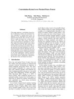
Figure 4 shows examples of the question classifi-
cation data used here.
question types input object : word sequences ([ ]: information of chunk and  : named entity)
ABBREVIATION what,[B-NP] be,[B-VP] the,[B-NP] abbreviation,[I-NP] for,[B-PP] Texas,[B-NP],B-GPE ?,[O]
DESCRIPTION what,[B-NP] be,[B-VP] Aborigines,[B-NP] ?,[O]
HUMAN who,[B-NP] discover,[B-VP] America,[B-NP],B-GPE ?,[O]
Figure 4: Examples of English question classification data
Table 3: Results of the Japanese question classification (F-measure)
(a) TIME TOP (b) LOCATION (c) ORGANIZATION (d) NUMEX

n
FSSK1
FSSK2
SK
BOW-K
1 2 3 4 ∞
- .961 .958 .957 .956
- .961 .956 .957 .956
- .946 .910 .866 .223
.902 .909 .886 .855 -
1 2 3 4 ∞
- .795 .793 .798 .792
- .788 .799 .804 .800
- .791 .775 .732 .169
.744 .768 .756 .747 -
1 2 3 4 ∞
- .709 .720 .720 .723
- .703 .710 .716 .720
- .705 .668 .594 .035
.641 690 .636 .572 -
1 2 3 4 ∞
- .912 .915 .908 .908
- .913 .916 .911 .913
- .912 .885 .817 .036
.842 .852 .807 .726 -
6.2 Sentence Modality Identification
For example, sentence modality identification tech-
niques are used in automatic text analysis systems
that identify the modality of a sentence, such as
“opinion” or “description”.

The data set was created from Mainichi news arti-
cles and one of three modality tags, “opinion”, “de-
cision” and “description” was applied to each sen-
tence. The data size was 1135 sentences consist-
ing of 123 sentences of “opinion”, 326 of “decision”
and 686 of “description”. We evaluated the results
by using 5-fold cross validation.
7 Results and Discussion
Tables 3 and 4 show the results of Japanese and En-
glish question classification, respectively. Table 5
shows the results of sentence modality identifica-
tion. n in each table indicates the threshold of the
sub-sequence size. n = ∞ means all possible sub-
sequences are used.
First, SK was consistently superior to BOW-K.
This indicates that the structural features were quite
efficient in performing these tasks. In general we
can say that the use of structural features can im-
prove the performance of NLP tasks that require the
details of the contents to perform the task.
Most of the results showed that SK achieves its
maximum performance when n = 2. The per-
formance deteriorates considerably once n exceeds
4. This implies that SK with larger sub-structures
degrade classification performance. These results
show the same tendency as the previous studies dis-
cussed in Section 3. Table 6 shows the precision and
recall of SK when n = ∞. As shown in Table 6, the
classifier offered high precision but low recall. This
is evidence of over-fitting in learning.

As shown by the above experiments, FSSK pro-
Table 6: Precision and recall of SK: n = ∞
Precision Recall F
MI:Opinion .917 .209 .339
JQA:LOCATION .896 .093 .168
vided consistently better performance than the con-
ventional methods. Moreover, the experiments con-
firmed one important fact. That is, in some cases
maximum performance was achieved with n =
∞. This indicates that sub-sequences created us-
ing very large structures can be extremely effective.
Of course, a larger feature space also includes the
smaller feature spaces, Σ
n
⊂ Σ
n+1
. If the perfor-
mance is improved by using a larger n, this means
that significant features do exist. Thus, we can im-
prove the performance of some classification prob-
lems by dealing with larger substructures. Even if
optimum performance was not achieved with n =
∞, difference between the performance of smaller
n are quite small compared to that of SK. This indi-
cates that our method is very robust as regards sub-
structure size; It therefore becomes unnecessary for
us to decide sub-structure size carefully. This in-
dicates our approach, using large sub-structures, is
better than the conventional approach of eliminating
sub-sequences based on size.

8 Conclusion
This paper proposed a statistical feature selection
method for convolution kernels. Our approach can
select significant features automatically based on a
statistical significance test. Our proposed method
can be embedded in the DP based kernel calcula-
tion process for convolution kernels by using sub-
structure mining algorithms.
Table 4: Results of English question classification (Accuracy)
(a) coarse (b) fine
n
FSSK1
FSSK2
SK
BOW-K
1 2 3 4 ∞
- .908 .914 .916 .912
- .902 .896 .902 .906
- .912 .914 .912 .892
.728 .836 .864 .858 -
1 2 3 4 ∞
- .852 .854 .852 .850
- .858 .856 .854 .854
- .850 .840 .830 .796
.754 .792 .790 .778 -
Table 5: Results of sentence modality identification (F-measure)
(a) opinion (b) decision (c) description
n
FSSK1
FSSK2

SK
BOW-K
1 2 3 4 ∞
- .734 .743 .746 .751
- .740 .748 .750 .750
- .706 .672 .577 .058
.507 .531 .438 .368 -
1 2 3 4 ∞
- .828 .858 .854 .857
- .824 .855 .859 .860
- .816 .834 .830 .339
.652 .708 .686 .665 -
1 2 3 4 ∞
- .896 .906 .910 .910
- .894 .903 .909 .909
- .902 .913 .910 .808
.819 .839 .826 .793 -
Experiments show that our method is superior to
conventional methods. Moreover, the results indi-
cate that complex features exist and can be effective.
Our method can employ them without over-fitting
problems, which yields benefits in terms of concept
and performance.
References
N. Cancedda, E. Gaussier, C. Goutte, and J M.
Renders. 2003. Word-Sequence Kernels. Jour-
nal ofMachine Learning Research, 3:1059–1082.
M. Collins and N. Duffy. 2001. Convolution Ker-
nels for Natural Language. In Proc. of Neural In-
formation Processing Systems (NIPS’2001).

C. Cortes and V. N. Vapnik. 1995. Support Vector
Networks. Machine Learning, 20:273–297.
D. Haussler. 1999. Convolution Kernels on Dis-
crete Structures. In Technical Report UCS-CRL-
99-10. UC Santa Cruz.
T. Joachims. 1998. Text Categorization with Sup-
port Vector Machines: Learning with Many Rel-
evant Features. In Proc. of European Conference
on Machine Learning (ECML ’98), pages 137–
142.
T. Kudo and Y. Matsumoto. 2002. Japanese Depen-
dency Analysis Using Cascaded Chunking. In
Proc. of the 6th Conference on Natural Language
Learning (CoNLL 2002), pages 63–69.
T. Kudo and Y. Matsumoto. 2003. Fast Methods for
Kernel-based Text Analysis. In Proc. of the 41st
Annual Meeting of the Association for Computa-
tional Linguistics (ACL-2003), pages 24–31.
X. Li and D. Roth. 2002. Learning Question Clas-
sifiers. In Proc. of the 19th International Con-
ference on Computational Linguistics (COLING
2002), pages 556–562.
H. Lodhi, C. Saunders, J. Shawe-Taylor, N. Cris-
tianini, and C. Watkins. 2002. Text Classification
Using String Kernel. Journal of Machine Learn-
ing Research, 2:419–444.
S. Morishita and J. Sese. 2000. Traversing Item-
set Lattices with Statistical Metric Pruning. In
Proc. of ACM SIGACT-SIGMOD-SIGART Symp.
on Database Systems (PODS’00), pages 226–

236.
J. Pei, J. Han, B. Mortazavi-Asl, and H. Pinto.
2001. PrefixSpan: Mining Sequential Patterns
Efficiently by Prefix-Projected Pattern Growth.
In Proc. of the 17th International Conference on
Data Engineering (ICDE 2001), pages 215–224.
M. Rogati and Y. Yang. 2002. High-performing
Feature Selection for Text Classification. In
Proc. of the 2002 ACM CIKM International Con-
ference on Information and Knowledge Manage-
ment, pages 659–661.
J. Suzuki, T. Hirao, Y. Sasaki, and E. Maeda.
2003a. Hierarchical Directed Acyclic Graph Ker-
nel: Methods for Natural Language Data. In
Proc. of the 41st Annual Meeting of the Associ-
ation for Computational Linguistics (ACL-2003),
pages 32–39.
J. Suzuki, Y. Sasaki, and E. Maeda. 2003b. Kernels
for Structured Natural Language Data. In Proc.
of the 17th Annual Conference on Neural Infor-
mation Processing Systems (NIPS2003).