Báo cáo khoa học: "Discourse Segmentation of Multi-Party Conversation" doc

Discourse Segmentation of Multi-Party Conversation
Michel Galley Kathleen McKeown
Columbia University
Computer Science Department
1214 Amsterdam Avenue
New York, NY 10027, USA
{galley,kathy}@cs.columbia.edu
Eric Fosler-Lussier
Columbia University
Electrical Engineering Department
500 West 120th Street
New York, NY 10027, USA

Hongyan Jing
IBM T.J. Watson Research Center
Yorktown Heights, NY 10598, USA

Abstract
We present a domain-independent topic
segmentation algorithm for multi-party
speech. Our feature-based algorithm com-
bines knowledge about content using a
text-based algorithm as a feature and
about form using linguistic and acous-
tic cues about topic shifts extracted from
speech. This segmentation algorithm uses
automatically induced decision rules to
combine the different features. The em-
bedded text-based algorithm builds on lex-
ical cohesion and has performance compa-
rable to state-of-the-art algorithms based

on lexical information. A significant er-
ror reduction is obtained by combining the
two knowledge sources.
1 Introduction
Topic segmentation aims to automatically divide text
documents, audio recordings, or video segments,
into topically related units. While extensive research
has targeted the problem of topic segmentation of
written texts and spoken monologues, few have stud-
ied the problem of segmenting conversations with
many participants (e.g., meetings). In this paper, we
present an algorithm for segmenting meeting tran-
scripts. This study uses recorded meetings of typi-
cally six to eight participants, in which the informal
style includes ungrammatical sentences and overlap-
ping speakers. These meetings generally do not have
pre-set agendas, and the topics discussed in the same
meeting may or may not related.
The meeting segmenter comprises two compo-
nents: one that capitalizes on word distribution to
identify homogeneous units that are topically cohe-
sive, and a second component that analyzes conver-
sational features of meeting transcripts that are in-
dicative of topic shifts, like silences, overlaps, and
speaker changes. We show that integrating features
from both components with a probabilistic classifier
(induced with c4.5rules) is very effective in improv-
ing performance.
In Section 2, we review previous approaches to
the segmentation problem applied to spoken and

written documents. In Section 3, we describe the
corpus of recorded meetings intended to be seg-
mented, and the annotation of its discourse structure.
In Section 4, we present our text-based segmenta-
tion component. This component mainly relies on
lexical cohesion, particularly term repetition, to de-
tect topic boundaries. We evaluated this segmenta-
tion against other lexical cohesion segmentation pro-
grams and show that the performance is state-of-the-
art. In the subsequent section, we describe conver-
sational features, such as silences, speaker change,
and other features like cue phrases. We present a
machine learning approach for integrating these con-
versational features with the text-based segmenta-
tion module. Experimental results show a marked
improvement in meeting segmentation with the in-
corporation of both sets of features. We close with
discussions and conclusions.
2 Related Work
Existing approaches to textual segmentation can be
broadly divided into two categories. On the one
hand, many algorithms exploit the fact that topic
segments tend to be lexically cohesive. Embodi-
ments of this idea include semantic similarity (Mor-
ris and Hirst, 1991; Kozima, 1993), cosine similarity
in word vector space (Hearst, 1994), inter-sentence
similarity matrix (Reynar, 1994; Choi, 2000), en-
tity repetition (Kan et al., 1998), word frequency
models (Reynar, 1999), or adaptive language models
(Beeferman et al., 1999). Other algorithms exploit

a variety of linguistic features that may mark topic
boundaries, such as referential noun phrases (Pas-
sonneau and Litman, 1997).
In work on segmentation of spoken docu-
ments, intonational, prosodic, and acoustic indica-
tors are used to detect topic boundaries (Grosz and
Hirschberg, 1992; Nakatani et al., 1995; Hirschberg
and Nakatani, 1996; Passonneau and Litman, 1997;
Hirschberg and Nakatani, 1998; Beeferman et al.,
1999; T
¨
ur et al., 2001). Such indicators include
long pauses, shifts in speaking rate, great range in
F0 and intensity, and higher maximum accent peak.
These approaches use different learning mecha-
nisms to combine features, including decision trees
(Grosz and Hirschberg, 1992; Passonneau and Lit-
man, 1997; T
¨
ur et al., 2001) exponential models
(Beeferman et al., 1999) or other probabilistic mod-
els (Hajime et al., 1998; Reynar, 1999).
3 The ICSI Meeting Corpus
We have evaluated our segmenter on the ICSI Meet-
ing corpus (Janin et al., 2003). This corpus is one of
a growing number of corpora with human-to-human
multi-party conversations. In this corpus, record-
ings of meetings ranged primarily over three differ-
ent recurring meeting types, all of which concerned
speech or language research.

1
The average duration
is 60 minutes, with an average of 6.5 participants.
They were transcribed, and each conversation turn
was marked with the speaker, start time, end time,
and word content.
From the corpus, we selected 25 meetings to be
segmented, each by at least three subjects. We
opted for a linear representation of discourse, since
finer-grained discourse structures (e.g. (Grosz and
Sidner, 1986)) are generally considered to be diffi-
cult to mark reliably. Subjects were asked to mark
each speaker change (potential boundary) as either
boundary or non-boundary. In the resulting anno-
tation, the agreed segmentation based on majority
1
While it would be desirable to have a broader variety of
meetings, we hope that experiments on this corpus will still
carry some generality.
opinion contained 7.5 segments per meeting on av-
erage, while the average number of potential bound-
aries is 770. We used Cochran’s Q (1950) to eval-
uate the agreement among annotators. Cochran’s
test evaluates the null hypothesis that the number
of subjects assigning a boundary at any position is
randomly distributed. The test shows that the inter-
judge reliability is significant to the 0.05 level for 19
of the meetings, which seems to indicate that seg-
ment identification is a feasible task.
2

4 Segmentation based on Lexical Cohesion
Previous work on discourse segmentation of written
texts indicates that lexical cohesion is a strong in-
dicator of discourse structure. Lexical cohesion is
a linguistic property that pertains to speech as well,
and is a linguistic phenomenon that can also be ex-
ploited in our case: while our data does not have
the same kind of syntactic and rhetorical structure
as written text, we nonetheless expect that informa-
tion from the written transcription alone should pro-
vide indications about topic boundaries. In this sec-
tion, we describe our work on LCseg, a topic seg-
menter based on lexical cohesion that can handle
both speech and text, but that is especially designed
to generate the lexical cohesion feature used in the
feature-based segmentation described in Section 5.
4.1 Algorithm Description
LCseg computes lexical chains, which are thought
to mirror the discourse structure of the underly-
ing text (Morris and Hirst, 1991). We ignore syn-
onymy and other semantic relations, building a re-
stricted model of lexical chains consisting of sim-
ple term repetitions, hypothesizing that major topic
shifts are likely to occur where strong term repeti-
tions start and end. While other relations between
lexical items also work as cohesive factors (e.g. be-
tween a term and its super-ordinate), the work on
linear topic segmentation reporting the most promis-
ing results account for term repetitions alone (Choi,
2000; Utiyama and Isahara, 2001).

The preprocessing steps of LCseg are common to
many segmentation algorithms. The input document
is first tokenized, non-content words are removed,
2
Four other meetings failed short the significance test, while
there was little agreement on the two last ones (p > 0.1).
and remaining words are stemmed using an exten-
sion of Porter’s stemming algorithm (Xu and Croft,
1998) that conflates stems using corpus statistics.
Stemming will allow our algorithm to more accu-
rately relate terms that are semantically close.
The core algorithm of LCseg has two main parts:
a method to identify and weight strong term repeti-
tions using lexical chains, and a method to hypothe-
size topic boundaries given the knowledge of multi-
ple, simultaneous chains of term repetitions.
A term is any stemmed content word within the
text. A lexical chain is constructed to consist of all
repetitions ranging from the first to the last appear-
ance of the term in the text. The chain is divided into
subchains when there is a long hiatus of h consecu-
tive sentences with no occurrence of the term, where
h is determined experimentally. For each hiatus, a
new division is made and thus, we avoid creating
weakly linked chains.
For all chains that have been identified, we use a
weighting scheme that we believe is appropriate to
the task of inducing the topical or sub-topical struc-
ture of text. The weighting scheme depends on two
factors:

Frequency: chains containing more repeated
terms receive a higher score.
Compactness: shorter chains receive a higher
weight than longer ones. If two chains of different
lengths contain the same number of terms, we assign
a higher score to the shortest one. Our assumption
is that the shorter one, being more compact, seems
to be a better indicator of lexical cohesion.
3
We apply a variant of a metric commonly used
in information retrieval, TF.IDF (Salton and Buck-
ley, 1988), to score term repetitions. If R
1
. . . R
n
is
the set of all term repetitions collected in the text,
t
1
. . . t
n
the corresponding terms, L
1
. . . L
n
their re-
spective lengths,
4
and L the length of the text, the
adapted metric is expressed as follows, combining

frequency (freq(t
i
)) of a term t
i
and the compact-
ness of its underlying chain:
score(R
i
) = f req(t
i
) · log(
L
L
i
)
3
The latter parameter might seem controversial at first, and
one might assume that longer chains should receive a higher
score. However we point out that in a linear model of dis-
course, chains that almost span the entire text are barely indica-
tive of any structure (assuming boundaries are only hypothe-
sized where chains start and end).
4
All lengths are expressed in number of sentences.
In the second part of the algorithm, we combine
information from all term repetitions to compute a
lexical cohesion score at each sentence break (or,
in the case of spoken conversations, speaker turn
break). This step of our algorithm is very similar
in spirit to TextTiling (Hearst, 1994). The idea is to

work with two adjacent analysis windows, each of
fixed size k. For each sentence break, we determine
a lexical cohesion function by computing the cosine
similarity at the transition between the two windows.
Instead of using word counts to compute similarity,
we analyze lexical chains that overlap with the two
windows. The similarity between windows (A and
B) is computed with:
5
cosine(A, B) =

i
w
i,A
·w
i,B


i
w
2
i,A

i
w
2
i,B
where
w
i,Γ

=

score(R
i
) if R
i
overlaps Γ ∈ {A, B}
0 otherwise
The similarity computed at each sentence break
produces a plot that shows how lexical cohesion
changes over time; an example is shown in Figure 1.
The lexical cohesion function is then smoothed us-
ing a moving average filter, and minima become po-
tential segment boundaries. Then, in a manner quite
similar to (Hearst, 1994), the algorithm determines
for every local minimum m
i
how sharp of a change
there is in the lexical cohesion function. The algo-
rithm looks on each side of m
i
for maxima of cohe-
sion, and once it eventually finds one on each side (l
and r), it computes the hypothesized segmentation
probability:
p(m
i
) =
1
2

[LCF(l) + LCF(r) − 2 · LCF(m)]
where LCF(x) is the value of the lexical cohesion
function at x.
This score is supposed to capture the sharpness of
the change in lexical cohesion, and give probabilities
close to 1 for breaks like sentence 179 in Figure 1.
Finally, the algorithm selects the hypothesized
boundaries with the highest computed probabilities.
If the number of reference boundaries is unknown,
the algorithm has to make a guess. It computes the
5
Normalizing anything in these windows has little ef-
fect, since the cosine similarity is scale invariant, that is
cosine(αx
a
, x
b
) = cosine(x
a
, x
b
) for α > 0.
20 40 60 80 100 120 140 160 180 200 220 240 260
0.2
0.3
0.4
0.5
0.6
0.7
0.8

0.9
1
Figure 1: Application of the LCseg algorithm on the concatenation of 16 WSJ stories. Numbers on the
x-axis represent sentence indices, and y-axis represents the lexical cohesion function. The representative
example presented here is segmented by LCseg with an error of P
k
= 15.79, while the average performance
of the algorithm is P
k
= 15.31 on the WSJ test corpus (unknown number of segments).
mean and the variance of the hypothesized probabil-
ities of all potential boundaries (local minima). As
we can see in Figure 1, there are many local minima
that do not correspond to actual boundaries. Thus,
we ignore all potential boundaries with a probability
lower than p
limit
. For the remaining points, we com-
pute the threshold using the average (µ) and standard
deviation (σ) of the p(m
i
) values, and each potential
boundary m
i
above the threshold µ−α·σ is hypoth-
esized as a real boundary.
4.2 Evaluation
We evaluate LCseg against two state-of-the-art seg-
mentation algorithms based on lexical cohesion
(Choi, 2000; Utiyama and Isahara, 2001). We use

the error metric P
k
proposed by Beeferman et al.
(1999) to evaluate segmentation accuracy. It com-
putes the probability that sentences k units (e.g. sen-
tences) apart are incorrectly determined as being ei-
ther in different segments or in the same one. Since
it has been argued in (Pevzner and Hearst, 2002) that
P
k
has some weaknesses, we also include results ac-
cording to the WindowDiff (WD) metric (which is
described in the same work).
A test corpus of concatenated
6
texts extracted
from the Brown corpus was built by Choi (2000)
to evaluate several domain-independent segmenta-
tion algorithms. We reuse the same test corpus for
our evaluation, in addition to two other test corpora
we constructed to test how segmenters scale across
genres and how they perform with texts with various
6
Concatenated documents correspond to reference seg-
ments.
number of segments.
7
We designed two test corpora,
each of 500 documents, using concatenated texts
extracted from the TDT and WSJ corpora, ranging

from 4 to 22 in number of segments.
LCseg depends on several parameters. Parameter
tuning was performed on three tuning corpora of one
thousand texts each.
8
We performed searches for the
optimal settings of the four tunable parameters in-
troduced above; the best performance was achieved
with h = 11 (hiatus length for dividing a chain into
parts), k = 2 (analysis window size), p
limit
= 0.1
and α =
1
2
(thresholding limits for the hypothesized
boundaries).
As shown in Table 1, our algorithm is signifi-
cantly better than (Choi, 2000) (labeled C99) on
all three test corpora, according to a one-sided t-
test of the null hypothesis of equal mean at the 0.01
level. It is not clear whether our algorithm is better
than (Utiyama and Isahara, 2001) (U00). When the
number of segments is provided to the algorithms,
our algorithm is significantly better than Utiyama’s
on WSJ, better on Brown (but not significant), and
significantly worse on TDT. When the number of
boundaries is unknown, our algorithm is insignifi-
cantly worse on Brown, but significantly better on
WSJ and TDT – the two corpora designed to have

a varying number of segments per document. In the
case of the Meeting corpus, none of the algorithms
are significantly different than the others, due to the
7
All texts in Choi’s test corpus have exactly 10 segments.
We are concerned that the adjustments of any algorithm param-
eters might overfit this predefined number of segments.
8
These texts are different from the ones used for evaluation.
Brown corpus
known unknown
P
k
W D P
k
W D
C99 11.19% 13.86% 12.07% 14.57%
U00 8.77% 9.44% 9.76% 10.32%
LCseg 8.69% 9.42% 10.49% 11.37%
p-val. 0.42 0.48 0.027 0.0037
TDT corpus
C99 9.37% 11.91% 10.18% 12.72%
U00 4.70% 6.29% 8.70% 11.12%
LCseg 6.15% 8.41% 6.95% 9.09%
p-val. 1.1e-05 2.8e-07 4.5e-05 2.8e-05
WSJ corpus
C99 19.61% 26.42% 22.32% 29.81%
U00 15.18% 21.54% 17.71% 24.06%
LCseg 12.21% 18.25% 15.31% 22.14%
p-val. 1.4e-08 1.7e-08 2.6e-04 0.0063

Meeting corpus
C99 33.79% 37.25% 47.42% 58.08%
U00 31.99% 34.49% 37.39% 40.43%
LCseg 26.37% 29.40% 31.91% 35.88%
p-val. 0.026 0.14 0.14 0.23
Table 1: Comparison C99 and U00. The p-values in
the table are the results of significance tests between
U00 and LCseg. Bold-faced values are scores that
are statistically significant.
small test set size.
In conclusion, LCseg has a performance compara-
ble to state-of-the-art text segmentation algorithms,
with the added advantage of computing a segmen-
tation probability at each potential boundary. This
information can be effectively used in the feature-
based segmenter to account for lexical cohesion, as
described in the next section.
5 Feature-based Segmentation
In the previous section, we have concentrated exclu-
sively on the consideration of content (through lexi-
cal cohesion) to determine the structure of texts, ne-
glecting any influence of form. In this section, we
explore formal devices that are indicative of topic
shifts, and explain how we use these cues to build a
segmenter targeting conversational speech.
5.1 Probabilistic Classifiers
Topic segmentation is reduced here to a classifica-
tion problem, where each utterance break B
i
is ei-

ther considered a topic boundary or not. We use
statistical modeling techniques to build a classifier
that uses local features (e.g. cue phrases, pauses)
to determine if an utterance break corresponds to
a topic boundary. We chose C4.5 and C4.5rules
(Quinlan, 1993), two programs to induce classifi-
cation rules in the form of decision trees and pro-
duction rules (respectively). C4.5 generates an un-
pruned decision tree, which is then analyzed by
C4.5rules to generate a set of pruned production
rules (it tries to find the most useful subset of them).
The advantage of pruned rules over decision trees is
that they are easier to analyze, and allow combina-
tion of features in the same rule (feature interactions
are explicit).
The greedy nature of decision rule learning algo-
rithms implies that a large set of features can lead
to bad performance and generalization capability. It
is desirable to remove redundant and irrelevant fea-
tures, especially in our case since we have little data
labeled with topic shifts; with a large set of fea-
tures, we would risk overfitting the data. We tried
to restrict ourselves to features whose inclusion is
motivated by previous work (pauses, speech rate)
and added features that are specific to multi-speaker
speech (overlap, changes in speaker activity).
5.2 Features
Cue phrases: previous work on segmentation has
found that discourse particles like now, well pro-
vide valuable information about the structure of texts

(Grosz and Sidner, 1986; Hirschberg and Litman,
1994; Passonneau and Litman, 1997). We analyzed
the correlation between words in the meeting cor-
pus and labeled topic boundaries, and automatically
extracted utterance-initial cue phrases
9
that are sta-
tistically correlated with boundaries. For every word
in the meeting corpus, we counted the number of its
occurrences near any topic boundary, and its num-
ber of appearances overall. Then, we performed χ
2
significance tests (e.g. figure 2 for okay) under the
null hypothesis that no correlation exists. We se-
lected terms whose χ
2
value rejected the hypothesis
under a 0.01-level confidence (the rejection criterion
is χ
2
≥ 6.635). Finally, induced cue phrases whose
usage has never been described in other work were
removed (marked with ∗ in Table 3). Indeed, there
is a risk that the automatically derived list of cue
phrases could be too specific to the word usage in
9
As in (Litman and Passonneau, 1995), we restrict ourselves
to the first lexical item of any utterance, plus the second one if
the first item is also a cue word.
Near boundary Distant

okay 64 740
Other 657 25896
Table 2: okay (χ
2
= 89.11, df = 1, p < 0.01).
okay 93.05 but 13.57
shall ∗ 27.34 so 11.65
anyway 23.95 and 10.99
we’re ∗ 17.67 should ∗ 10.21
alright 16.09 good ∗ 7.70
let’s ∗ 14.54
Table 3: Automatically selected cue phrases.
these meetings.
Silences: previous work has found that ma-
jor shifts in topic typically show longer silences
(Passonneau and Litman, 1993; Hirschberg and
Nakatani, 1996). We investigated the presence of
silences in meetings and their correlation with topic
boundaries, and found it necessary to make a distinc-
tion between pauses and gaps (Levinson, 1983). A
pause is a silence that is attributable to a given party,
for example in the middle of an adjacency pair, or
when a speaker pauses in the middle of her speech.
Gaps are silences not attributable to any party, and
last until a speaker takes the initiative of continuing
the discussion. As an approximation of this distinc-
tion, we classified a silence that follows a question or
in the middle of somebody’s speech as a pause, and
any other silences as a gap. While the correlation be-
tween long silences and discourse boundaries seem

to be less pervasive in meetings than in other speech
corpora, we have noticed that some topic boundaries
are preceded (within some window) by numerous
gaps. However, we found little correlation between
pauses and topic boundaries.
Overlaps: we also analyzed the distribution of
overlapping speech by counting the average overlap
rate within some window. We noticed that, many
times, the beginning of segments are characterized
by having little overlapping speech.
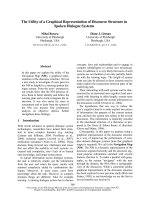
Speaker change: we sometimes noticed a corre-
lation between topic boundaries and sudden changes
in speaker activity. For example, in Figure 2, it
is clear that the contribution of individual speakers
to the discussion can greatly change from one dis-
course unit to the next. We try to capture significant
changes in speakership by measuring the dissimilar-
ity between two analysis windows. For each poten-
tial boundary, we count for each speaker i the num-
ber of words that are uttered before (L
i
) and after
(R
i
) the potential boundary (we limit our analysis
to a window of fixed size). The two distributions
are normalized to form two probability distributions
l and r, and significant changes of speakership are
detected by computing their Jensen-Shannon diver-
gence:

JS(l, r) =
1
2
[D(l||avg
l,r
) + D(r||avg
l,r
)]
where D(l||r) is the KL-divergence between the
two distributions.
Lexical cohesion: we also incorporated the lexi-
cal cohesion function computed by LCseg as a fea-
ture of the multi-source segmenter in a manner simi-
lar to the knowledge source combination performed
by (Beeferman et al., 1999) and (T
¨
ur et al., 2001).
Note that we use both the posterior estimate com-
puted by LCseg and the raw lexical cohesion func-
tion as features of the system.
5.3 Features: Selection and Combination
For every potential boundary B
i
, the classifier ana-
lyzes features in a window surrounding B
i
to decide
whether it is a topic boundary or not. It is generally
unclear what is the optimal window size and how
features should be analyzed. Windows of various

sizes can lead to different levels of prediction, and
in some cases, it might be more appropriate to only
extract features preceding or following B
i
.
We avoided making arbitrary choices of parame-
ters; instead, for any feature F and a set F
1
, . . . , F
n
of possible ways to measure the feature (different
window sizes, different directions), we picked the F
i
that is in isolation the best predictor of topic bound-
aries (among F
1
, . . . , F
n
). Table 4 presents for each
feature the analysis mode that is the most useful on
the training data.
5.4 Evaluation
We performed 25-fold cross-validation for evaluat-
ing the induced probabilistic classifier, computing
the average of P
k
and W D on the held-out meet-
ings. Feature selection and decision rule learning
0 10 20 30
Figure 2: speaker activity in a meeting. Each row represent the speech activity of one speaker, utterance of

words being represented as black. Vertical lines represent topic shifts. The x-axis represents time.
Feature Tag Size (sec.) Side
Cue phrases CUE 5 both
Silence (gaps) SIL 30 left
Overlap† OVR 30 right
Speaker activity ACT 5 both
Lexical cohesion LC 30 both
†: the size of the window that was used to compute the
JS-divergence was also determined automatically.
Table 4: Parameters for feature analysis.
is always performed on sets of 24 meetings, while
the held-out data is used for testing. Table 5 gives
some examples of the type of rules that are learned.
The first rule states that if the value for the lexical
cohesion (LC) function is low at the current sen-
tence break, there is at least one CUE phrase, there
is less than three seconds of silence to the left of the
break,
10
and a single speaker holds the floor for a
longer period of time than usual to the right of the
break, then we have a topic break. In general, we
found that the derived rules show that lexical cohe-
sion plays a stronger role than most other features
in determining topic breaks. Nonetheless, the quan-
titative results summarized in table 6, which corre-
spond to the average performance on the held-out
sets, show that the integration of conversational fea-
tures with the text-based segmenter outperforms ei-
ther alone.

6 Conclusions
We presented a domain-independent segmentation
algorithm for multi-party conversation that inte-
grates features based on content with features based
on form. The learned combination of features results
in a significant increase in accuracy over previous
10
Note that rules are not always meaningful in isolation and
it is likely that a subordinate rule in the tree to this one would do
further tests on silence to determine if a topic boundary exists.
Condition Decision Conf.
LC ≤ 0.67, CUE ≥ 1,
OVR ≤ 1.20, SIL ≤ 3.42 yes 94.1
LC ≤ 0.35, SIL > 3.42,
OVR ≤ 4.55 yes 92.2
CUE ≥ 1, ACT > 0.1768,
OVR ≤ 1.20, LC ≤ 0.67 yes 91.6
. . .
default no
Table 5: A selection of the most useful rules learned
by C4.5rules along with their confidence levels.
Times for OVR and SIL are expressed in seconds.
P
k
W D
feature-based 23.00% 25.47%
LCseg 31.91% 35.88%
U00 37.39% 40.43%
p-value 2.14e-04 3.30e-04
Table 6: Performance of the feature-based seg-

menter on the test data.
approaches to segmentation when applied to meet-
ings. Features based on form that are likely to in-
dicate topic shifts are automatically extracted from
speech. Content based features are computed by a
segmentation algorithm that utilizes a metric of lex-
ical cohesion and that performs as well as state-of-
the-art text-based segmentation techniques. It works
both with written and spoken texts. The text-based
segmentation approach alone, when applied to meet-
ings, outperforms all other segmenters, although the
difference is not statistically significant.
In future work, we would like to investigate the
effects of adding prosodic features, such as pitch
ranges, to our segmenter, as well as the effect of
using errorful speech recognition transcripts as op-
posed to manually transcribed utterances.
An implementation of our lexical cohesion seg-
menter is freely available for educational or research
purposes.
11
Acknowledgments
We are grateful to Julia Hirschberg, Dan Ellis, Eliz-
abeth Shriberg, and Mari Ostendorf for their helpful
advice. We thank our ICSI project partners for grant-
ing us access to the meeting corpus and for useful
discussions. This work was funded under the NSF
project Mapping Meetings (IIS-012196).
References
D. Beeferman, A. Berger, and J. Lafferty. 1999. Statisti-

cal models for text segmentation. Machine Learning,
34(1–3):177–210.
F. Choi. 2000. Advances in domain independent linear
text segmentation. In Proc. of NAACL’00.
W. Cochran. 1950. The comparison of percentages in
matched samples. Biometrika, 37:256–266.
B. Grosz and J. Hirschberg. 1992. Some intonational
characteristics of discourse structure. In Proc. of
ICSLP-92, pages 429–432.
B. Grosz and C. Sidner. 1986. Attention, intentions and
the structure of discourse. Computational Linguistics,
12(3).
M. Hajime, H. Takeo, and O. Manabu. 1998. Text seg-
mentation with multiple surface linguistic cues. In
COLING-ACL, pages 881–885.
M. Hearst. 1994. Multi-paragraph segmentation of ex-
pository text. In Proc. of the ACL.
J. Hirschberg and D. Litman. 1994. Empirical studies
on the disambiguation of cue phrases. Computational
Linguistics, 19(3):501–530.
J. Hirschberg and C. Nakatani. 1996. A prosodic anal-
ysis of discourse segments in direction-giving mono-
logues. In Proc. of the ACL.
J. Hirschberg and C. Nakatani. 1998. Acoustic indicators
of topic segmentation. In Proc. of ICSLP.
A. Janin, D. Baron, J. Edwards, D. Ellis, D. Gelbart,
N. Morgan, B. Peskin, T. Pfau, E. Shriberg, A. Stol-
cke, and C. Wooters. 2003. The ICSI meeting corpus.
In Proc. of ICASSP-03, Hong Kong (to appear).
11

/>M Y. Kan, J. Klavans, and K. McKeown. 1998. Linear
segmentation and segment significance. In Proc. 6th
Workshop on Very Large Corpora (WVLC-98).
H. Kozima. 1993. Text segmentation based on similarity
between words. In Proc. of the ACL.
S. Levinson. 1983. Pragmatics. Cambridge University
Press.
D. Litman and R. Passonneau. 1995. Combining multi-
ple knowledge sources for discourse segmentation. In
Proc. of the ACL.
J. Morris and G. Hirst. 1991. Lexcial cohesion computed
by thesaural relations as an indicator of the structure of
text. Computational Linguistics, 17:21–48.
C. Nakatani, J. Hirschberg, and B. Grosz. 1995. Dis-
course structure in spoken language: Studies on
speech corpora. In AAAI-95 Symposium on Empirical
Methods in Discourse Interpretation.
R. Passonneau and D. Litman. 1993. Intention-based
segmentation: Human reliability and correlation with
linguistic cues. In Proc. of the ACL.
R. Passonneau and D. Litman. 1997. Discourse seg-
mentation by human and automated means. Compu-
tational Linguistics, 23(1):103–139.
L. Pevzner and M. Hearst. 2002. A critique and im-
provement of an evaluation metric for text segmenta-
tion. Computational Linguistics, 28 (1):19–36.
R. Quinlan. 1993. C4.5: Programs for Machine Learn-
ing. Machine Learning. Morgan Kaufmann.
J. Reynar. 1994. An automatic method of finding topic
boundaries. In Proc. of the ACL.

J. Reynar. 1999. Statistical models for topic segmenta-
tion. In Proc. of the ACL.
G. Salton and C. Buckley. 1988. Term weighting ap-
proaches in automatic text retrieval. Information Pro-
cessing and Management, 24(5):513–523.
G. T
¨
ur, D. Hakkani-T
¨
ur, A. Stolcke, and E. Shriberg.
2001. Integrating prosodic and lexical cues for auto-
matic topic segmentation. Computational Linguistics,
27(1):31–57.
M. Utiyama and H. Isahara. 2001. A statistical model
for domain-independent text segmentation. In Proc. of
the ACL.
J. Xu and B. Croft. 1998. Corpus-based stemming using
cooccurrence of word variants. ACM Transactions on
Information Systems, 16(1):61–81.