Báo cáo khoa học: "Classifying Recognition Results for Spoken Dialog Systems" doc

Classifying Recognition Results for Spoken Dialog Systems
Malte Gabsdil
Deptartment of Computational Linguistics
Saarland University
Germany

Abstract
This paper investigates the correlation be-
tween acoustic confidence scores as re-
turned by speech recognizers with recog-
nition quality. We report the results of two
machine learning experiments that predict
the word error rate of recognition hypothe-
ses and the confidence error rate for indi-
vidual words within them.
1 Introduction
Acoustic confidence scores as computed by speech
recognizers play an important role in the design of
spoken dialog systems. Often, systems solely de-
cide on the basis of an overall acoustic confidence
score whether they should accept (consider correct),
clarify (ask for confirmation), or reject (prompt for
repeat/rephrase) the interpretation of an user utter-
ance. This behavior is usually achieved by setting
two fixed confidence thresholds: if the confidence
score of an utterance is above the upper threshold it
is accepted, when it is below the lower threshold it is
rejected, and clarification is initiated in case the con-
fidence score lies in between the two thresholds. The
GoDiS spoken dialog system (Larsson and Ericsson,
2002) is an example of such a system. More elabo-

rated and flexible system behavior can be achieved
by making use of individual word confidence scores
or slot-confidences
1
that allow more fine-grained de-
1
Some recognition platforms allow the application program-
mer to associate semantic slot values with certain words of
an input utterance. The slot-confi dence is then defi ned as the
acoustic confi dence for the words that make up this slot.
cisions as to which parts of an utterance are not suf-
ficiently well understood.
The aim of this paper is to investigate how
well acoustic confidences correlate with recognition
quality and to use machine learning (ML) techniques
to improve this correlation. In particular, we will
conduct two different experiments. First, we try
to predict the word error rate (WER) of a recogni-
tion result based on its overall confidence score and
show that we can improve on this by using ML clas-
sifiers. Second, we will consider individual word
confidence scores and again show that ML tech-
niques can be fruitfully applied to the task of decid-
ing whether individual words were recognized cor-
rectly or not.
The paper is organized as follows. In the next sec-
tion, we explain the general experimental setup, in-
troduce acoustic confidences, and explain how we
labeled our data. Sections 3 and 4 report on the ac-
tual experiments. Section 5 summarizes and con-

cludes the paper.
2 Experimental Setup
We use the ATIS2 corpus (MADCOW, 1992) as our
speech data source. The corpus contains approx.
15.000 utterances and has a vocabulary size of about
1.000 words. In order to get “real” recognition data,
we trained and tested the commercial NUANCE8.0
2
recognition engine on the ATIS2 corpus. To this end
we first split the corpus into two distinct sets. With
the first set we trained a statistical language model
(trigram) for the recognizer. This model was then
2

used to recognize the other set of utterances (using
1-best recognition). Finally, we split the set of rec-
ognized utterances into three different sets. A train-
ing set (75%), a test set (20%) and a development
set (5%).
2.1 Acoustic Confidences
The NUANCE recognizer returns an overall acous-
tic confidence score for each recognition hypothe-
sis as well as individual word confidence scores for
each word in the hypothesis. Acoustic confidences
are computed in an additional step after the actual
recognition process. The aim is to estimate a nor-
malized probability of a (sub-)sequence of words
that can be interpreted as a predictor whether the se-
quence was correctly recognized or not (see (Wessel
et al., 2001) for a comparison of different confidence

estimators). Acoustic confidence scores are there-
fore different from the unnormalized scores com-
puted by the standard Viterbi decoding in HMM
based recognition which selects the best hypothesis
among competing alternatives.
We will use acoustic confidence scores to derive
baseline values for the two experiments reported in
Sections 3 and 4.
2.2 Recognition Results
We first give a general overview of the performance
of the NUANCE speech recognizer. Table 1 reports
the overall word error rate (WER) in terms of inser-
tions, deletions, and substitutions as computed by
the recognition engine (but see the discussion on the
Levenstein distance in the next paragraph).
Insertions
Deletions Substitutions WER
1342 1693 5856 11.83
Table 1: Overall WER
Table 2 shows the absolute number and percent-
ages of the sentences that where recognized cor-
rectly (WER0), recognized with a WER between
1% and 50% (WER50), and with a WER greater
than 50% (WER100). Rejections and timeouts refer
to the number of utterances completely rejected by
the recognizer and utterances for which a process-
ing timeout threshold was exceeded. In both cases
the recognizer did not return a hypothesis.
Abs. Perc.
WER0 3824 51.0%

WER50
3204 42.7%
WER100
283 3.8%
Rejections 5 0.1%
Timeouts
187 2.5%
Total 7503 100.1%
Table 2: Recognition results grouped by WER
In our first experiment we will use the three cate-
gories WER0, WER50, and WER100 to establish a
correlation between the overall acoustic confidence
score for an utterance and its word error rate. The
basic idea is that these three classes might be used
by a system to decide whether it should accept, clar-
ify, or reject an hypothesis.
2.3 Labeling Words
We also labeled each word in the set of recognized
utterances as either correctly or incorrectly recog-
nized. The labeling is based on the Levenstein dis-
tance between the actual transcription of an utter-
ance and its recognition hypothesis. The Leven-
stein distance computes an alignment that minimizes
the number of insertions, deletions, and substitutions
when comparing two different sentences. However,
this distance can be ambiguous between two or more
alignment transcripts (i.e. there are can be several
ways to convert one string into another using the
minimum number of insertions, deletions, and sub-
stitutions). (1) shows two possible alignments for a

recognized utterance from the ATIS2 corpus, where
‘m’ stands for match, ‘i’ for insertion, and ‘s’ for
substitution.
(1) Ambiguous Levenstein alignment
Trans: are there any stops on that flight
Recog: what are the stops on the flight
Align1: s-s-s-m-m-s-m
Align2: i-m-s-d-m-m-s-m
To avoid this kind of ambiguity, we converted
all words to their phoneme representations using
the CMU pronunciation dictionary
3
. We then ran
3
/>cmudict
the Levenstein distance algorithm on these repre-
sentations and converted back the result to the word
level. This procedure gives us more intuitive align-
ment results because it has a bias towards substi-
tuting phonemically similar words (e.g. Align2 in
(1) above). Of course, the Levenstein distance on
the phoneme level can again be ambiguous but this
is more unlikely since the to-be aligned strings are
longer.
We will use the individually labeled words in our
second experiment where we try to improve the con-
fidence error rate and the detection-error tradeoff
curve for the recognition results.
3 Experiment 1
The purpose of the first experiment was to find out

how well features that can be automatically derived
from a recognition hypothesis can be used to predict
its word error rate.
As already mentioned in the previous section, all
recognized sentences were assigned to one of the
following classes depending on their actual WER:
WER0 (WER 0%, sentence correctly recognized),
WER50 (sentences with a WER between 1% and
50%), and WER100 (sentences with a WER greater
than 50%). The motivation to split the data into these
three classes was that they can be associated with the
two fixed thresholds commonly used in spoken dia-
log systems to decide whether an utterance should
be accepted, clarified, or rejected.
We are aware that this might not be an optimal
setting. Some spoken dialog systems only spot for
keywords or key-phrases in an utterance. For them it
does not matter whether “unimportant” words were
recognized correctly or not and a WER greater than
zero is often acceptable. The main problem is that
what counts as a keyword or key-phrase is system
and domain depended. We cannot simply base our
experiments on the WER for content words like
nouns, verbs, and adjectives. In a travel agency
application, for example, the prepositions ‘to’ and
‘from’ are quite important. In home automation,
quantifiers/determiners are important to distinguish
between the commands ‘switch off all lights’ and
‘switch off the hall lights’ (this example is borrowed
from David Milward). For further examples see also

(Bos and Oka, 2002).
3.1 Machine Learners
We predicted the WER-class for recognized sen-
tences based on their overall confidence score, and
with the two machine learners TiMBL (Daelemans
et al., 2002) and Ripper (Cohen, 1996). TiMBL
is a software package that provides two different
memory based learning algorithms, each with fine-
tunable metrics. All our TiMBL experiments were
done with the IB1 algorithm that uses the k-nearest
neighbor approach to classification: the class of a
test item is derived from the training instances that
are most similar to it. Memory-based learning is
often referred to as “lazy” learning because it ex-
plicitly stores all training examples in memory with-
out abstracting away from individual instances in the
learning process.
Ripper, on the other hand, implements a “greedy”
learning algorithm that tries to find regularities in the
training data. It induces rule sets for each class with
built-in heuristics to maximize accuracy and cover-
age. With default settings, rules are first induced
for low frequency classes, leaving the most frequent
class being the default. We chose TiMBL and Rip-
per as our two machine learners because they em-
ploy different approaches to classification, are well-
known, and widely available.
For all experiments we proceeded as follows:
First we used the training set to learn optimal con-
fidence thresholds for the baseline classification and

the development set to learn program parameters for
the two machine learners, which were then trained
on the training set. We then tested these settings on
the test set. To be able to statistically compare the
results, in a third step, we used the learned program
parameters to classify the recognition results in the
combined training and test sets in a 10-fold cross-
validation experiment. The optimization and evalu-
ation were always done on the weighted f
.5
-score
4
for all three classes.
3.2 Baseline
As a baseline predictor for class assignment we use
the overall confidence score of a recognition result
returned by the NUANCE recognizer. To assign the
three different classes, we have to learn two confi-
4
f
.5
is the unbiased harmonic mean of precision (p) and re-
call (r): f
.5
= 2pr/(p + r)
dence thresholds. Whenever the overall confidence
of the recognition result is below the lower thresh-
old, we classify it as WER100, whenever it is above
the upper threshold we classify it as WER0, and
when it is between we classify it as WER50. We

report the weighted f
.5
-score for the test set and the
cross-validation experiment as well as the standard
deviation for the cross-validation experiment in Ta-
ble 3.
Weighted f
.5
St. Deviation
test set 63.57% –
crossval
64.13% 1.67
Table 3: Baseline results
The confidence scores that maximized the results
for the NUANCE recognizer on the test set were 66
and 43.
3.3 ML Classification
We computed a feature vector representation for
each recognition result which served as input for
the two machine learners TiMBL and Ripper. Al-
together, 27 features were automatically extracted
from the recognizer output and the wave-form files
of the individual utterances. These features can
be grouped into the following seven different cate-
gories.
1. Recognizer Confidences: Overall confidence
score, max., min., and range of individual
word confidences, descriptive statistics of the
individual word confidences
2. Hypothesis Length: Length of audio sample,

number of words, syllables, and phonemes
(CMU based) in recognition hypothesis
3. Tempo: Length of audio sample divided by
the number of words, phones, and syllables
4. Recognizer Statistics: Time needed for de-
coding
5. Site Information: At which site the speech file
was recorded
5
6. f0 Statistics: Mean and max. f0, variance,
standard deviation, and number of unvoiced
frames
6
7. RMS Statistics: Mean and max. RMS, vari-
ance, standard deviation, number of frames
with RMS < 100
Automatic classification of the recognition re-
sults was done with different parameter and fea-
ture settings for the machine learners. We hereby
coarsely followed (Daelemans and Hoste, 2002)
who showed that parameter optimization and fea-
ture selection techniques improved classification re-
sults with TiMBL and Ripper for a variety of dif-
ferent tasks. First, both learners were run with their
default settings. Second, we optimized the param-
eters for the two learners on the development set.
Finally, we used a forward feature selection algo-
rithm interleaved with parameter optimization for
TiMBL. This algorithm starts out with zero features,
adds one feature, and performs parameter optimiza-

tion. This is done for all features and the five best
results are stored. The algorithm then iterates and
adds a second feature to these five best parameter
settings. Again, parameter optimization is done for
every possible feature combination. The algorithm
stops when there is no improvement for either of the
five best candidates when adding an additional fea-
ture. Keeping the five best parameter settings en-
sures that the feature selection is not too greedy. If,
for example, a single feature gives good results but
the combination with other features leads to a drop
in performance, there is still a change that, say, the
second or third best feature from the previous itera-
tion combines well with a new feature and leads to
better results.
We report the results for TiMBL (Table 4) and
Ripper (Table 5), respectively.
Weighted f
.5
St. Deviation
Default Settings
test set
60.44% –
crossval
61.24% 1.46
Parameter Optimization
test set
68.44% –
crossval
68.59% 2.03

Feature Selection
test set
66.41% –
crossval
67.01% 2.14
Table 4: TiMBL results
5
The ATIS2 data was recorded at several different sites.
6
The f0 and RMS (root mean square; a measure of the signal
energy level) features were extracted with Entropic’s get f0 tool.
Weighted f
.5
St. Deviation
Default Settings
test set
67.97% –
crossval
68.60% 1.54
Parameter Optimization
test set
68.11% –
crossval
68.23% 1.46
Table 5: Ripper results
The results show that TiMBL profits from param-
eter optimization and feature selection. One reason
for this is that, with default settings, TiMBL only
considers the nearest neighbor in deciding which
class to assign to a test item. In our experiment, con-

sidering more than one neighbor lead to a better f
.5
-
score for the majority class (WER0) which in turn
had an impact on overall weighted f
.5
-score. A sur-
prising finding is that the feature selection algorithm
did not lead to an improvement. We expected a bet-
ter score based on (Daelemans and Hoste, 2002) and
because some aspects in the feature vector specifi-
cation (e.g. tempo) are heavily correlated which can
cause problems for memory based learners. How-
ever, it turned out that our algorithm stopped after
selecting only seven of the 27 features which indi-
cates that it might still be too greedy. Another ex-
planation for the results is that optimization with
feature selection can be particularly prone to over-
fitting: The weighted f
.5
-score for the development
data, which we used to select features and optimize
parameters, was 77.40% (almost 11% better than the
performance on the test set).
Parameter optimization did not improve the re-
sults for Ripper. Compared to TiMBL the smaller
standard deviation in the cross-validation results in-
dicates a more uniform/stable classification of the
data.
3.4 Significance

We used related t-tests and Wilcoxon signed ranks
statistics to compare the cross-validation results. All
test were done two-tailed at a significance level of
p = .01. We found that the results for TiMBL
with default settings are significantly worse than all
other results. The other four machine learning re-
sults (parameter optimization and feature selection
for TiMBL as well as defaults and parameter op-
timization for Ripper) significantly outperform the
baseline. We could not find a significant differ-
ence between the TiMBL (excluding default set-
tings) and Ripper results. In all comparisons, t-test
and Wilcoxon signed ranks lead to the same results.
3.5 Ripper Rule Inspection
During learning, Ripper generates a set of (human
readable) decision rules that indicate which features
were most important in the classification process.
We cannot give a detailed analysis of the induced
rules because of space constraints, but Table 6 pro-
vides a simple breakdown by feature groups that
shows how often features from each group appeared
in the rule set.
7
1. Recognizer Confidences: 25
2. Hypothesis Length: 12
3. Tempo: 1
4. Recognizer Statistics: 8
5. Site Information: 0
6. f0 Statistics: 3
7. RMS Statistics: 2

Table 6: Features used by Ripper
We can see that all feature groups except “Site
Information” contribute to the rule set. The single
most often used feature was the mean of all individ-
ual word confidences (9 times), followed by the min-
imum individual word confidence and recognizer la-
tency (both 8 times). The overall acoustic confi-
dence score appeared in 4 rules only.
4 Experiment 2
The aim of the second experiment was to investigate
whether we can improve the confidence error rate
(CER) for the recognized data. The CER measures
how good individual word confidence scores predict
whether words are correctly recognized or not. A
confidence threshold is set according to which all
words are either tagged as correct or incorrect. The
7
The fi gures reported in Table 6 were obtained by training
Ripper on the training set with default parameters. Altogether,
16 classifi cation rules were generated.
CER is then simply defined as the number of in-
correctly assigned tags divided by the total num-
ber of recognized words. The CER is a very sim-
ple measure that strongly depends on the tagging
threshold and the prior probability of the classes cor-
rect and incorrect. Since we have a strong bias to-
wards correct words in our data, we complement the
CER evaluation with a second evaluation matrix, the
detection-error tradeoff (DET) curve which plots the
false acceptance rate (the number of incorrect words

tagged as correct divided by the total number of in-
correct words) over the false rejection rate (the num-
ber of correct words tagged as incorrect divided by
the total number of correct words). This curve is
instructive because it shows the results for several
different tagging thresholds and how they effect the
prediction accuracy for the two classes.
4.1 Features
The feature vector for the machine learners in the
second experiment consisted of 17 features which
were automatically derived from the recognition re-
sults and the output of Experiment 1. We can again
group them into different categories.
1. Overall Confidence: Overall confidence score
of the hypothesis the to-be-classified word ap-
pears in
2. Left word context: The two word forms left of
the to-be-classified word and their individual
word confidence scores
3. Word: The to-be-classified word from, its
individual word confidence, and two length
measures
4. Right word context: The two word forms left
of the to-be-classified word and their individ-
ual word confidence scores
5. WER estimate: The WER class as assigned to
the sentence the to-be-classified word appears
in based on the best results from Experiment 1
6. Sentence Length: Three different length mea-
sures for the recognition hypothesis the to-be-

classified word appears in
4.2 Confidence Error Rates
We report the confidence error rates for the test set
and cross-validation on the combined train and test
sets in Table 7. The machine learners were only run
with their default settings.
CER St. Deviation
Baseline
test set
11.47% –
crossval
11.23% 0.67
TiMBL
test set
11.44% –
crossval
11.30% 0.55
Ripper
test set
13.17% –
crossval
10.82% 0.68
Table 7: CER results
As in Experiment 1, we used related t-tests and
Wilcoxon signed ranks statistics to compare the re-
sults. Unfortunately, we could not find a significant
improvement for the machine learners as compared
to the baseline. Both tests show that there is no sig-
nificant difference between either of the three results
for two tailed tests at p = .01. Note, however, that

the CER is strongly dependent on the prior probabil-
ities of the classes correct and incorrect. It is there-
fore interesting to compare the performance on the
minority class (incorrect) for the baseline, TiMBL,
and Ripper. Table 8 shows precision, recall, and f
.5
-
scores on the test set.
prec recall f
.5
baseline 56.93 8.90 15.39
TiMBL
51.79 35.54 42.15
Ripper
50.84 27.55 35.74
Table 8: Minority class classification
We can see that the baseline performs very poor
on the minority class. Indeed the optimal thresh-
old computed during training was 15 which means
that almost every word is tagged as correct. This
difference does not show up in the CER because it
is “overshadowed” by the majority class. The next
paragraph will show the advantage of the machine
learners when we give equal weight to both the ma-
jority and minority classes.
4.3 Detection-Error Tradeoff
We use the data from all words in the training and
test sets to plot detection-error tradeoff curves. To
get the baseline DET curve (based on the individual
word confidence computed by the NUANCE recog-

nizer) we simply vary the tagging threshold between
100 and 0 and apply it to the data. A threshold of
50, for example, will classify all words with a con-
fidence higher or equal than 50 as correct and all
others as incorrect. The result is a gradual decline in
the false rejection rate: When the threshold is 100,
all instances will be tagged as incorrect, when it is
0, all instances will be tagged as correct.
4.4 Training Set Composition
We classified the same data with the machine learn-
ers using several 5-fold cross-validation experi-
ments. One big obstacle with the machine learn-
ers was that we wanted to force them to gradually
produce more false acceptances and less false rejec-
tions. Ripper provides a parameter to change the
“loss ratio”, i.e the ratio of the cost of a false neg-
ative to the cost of a false positive. This is exactly
what we want but we found that we cannot linearly
vary this parameter in a way that gives us a smooth
transition between false acceptances and false rejec-
tions.
We solved this problem by conducting experi-
ments were we changed the ratio of examples from
the two classes within the training set. This was
done as follows. During cross-validation we first
set aside an equal number of examples from both
classes from the training set. Depending on the ra-
tio value, we then added a certain fraction of one of
these two sets to the other set. For example, to get a
50/50 ratio, we simply combined the two sets; for a

75/25 ratio we took the first set and added to it 50%
(randomly selected) items from the second set. This
procedure in itself does not ensure a smooth transi-
tion from false rejections to false acceptances but it
worked very well in practice. Note that we basically
only take out a certain number of elements from the
cross-validation training set. We do still test every
data point since we do not change the ratio within
the test sets.
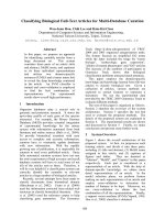
Figures 1 and 2 show the DET curves for TiMBL
and Ripper as compared to the baseline respectively.
4.5 Results
The DET curve for TiMBL is almost identical to the
baseline. The curve for Ripper, however, does im-
0
0.2
0.4
0.6
0.8
1
0 0.2 0.4 0.6 0.8 1
False rejection rate
False acceptance rate
"Baseline"
"TiMBL"
Figure 1: DET for TiMBL
0
0.2
0.4
0.6

0.8
1
0 0.2 0.4 0.6 0.8 1
False rejection rate
False acceptance rate
"Baseline"
"Ripper"
Figure 2: DET for Ripper
prove over the baseline, especially for false accep-
tance rates (FAR) up to 0.5. This is an interesting
finding because we are often interested in a good
performance for the minority class without loosing
too much accuracy on the majority class. For spoken
dialog systems it is of major importance to be “con-
servative” and to spot most of the erroneous words
in order to avoid misunderstandings. But this is al-
ways at the cost of inefficient and annoying dialogs
where the system rejects too many utterances or asks
too many clarification questions. Figure 2 shows
an improvement on the part of the curve where the
FAR is low (i.e. where not many erroneous words
are accepted). For a FAR of 20% (i.e. only every
fifth incorrect word is not detected as such) Ripper
improves the false rejection rate (FRR) by 10% as
compared to the baseline. Figure 2 also shows an
improvement in the equal error rate (the point where
FAR and FFR are the same) from 28,5% to 25%.
4.6 Ripper Rule Inspection
Again, we can investigate the rule sets generated by
Ripper to find out which features were particularly

useful for classification. In Table 9, we report a
breakdown by feature groups for one of the cross-
validation folds that lead to a FAR of about 20% and
a FRR of about 30.5% (i.e. one of the data points
that showed the highest improvement over the base-
line). The rule set included 15 different rules.
1. Overall Confidence: 7
2. Left word context: 16
3. Word: 21
4. Right word context: 8
5. WER estimate: 2
6. Sentence Length: 3
Table 9: Features used by Ripper
Table 9 shows that features from all six feature
groups were used for classification. The single most
often used feature was the individual word confi-
dence of the target word (used in all rules), followed
by the word confidence of the immediately preceed-
ing word (which appeared in 11 rules).
5 Conclusions
Spotting erroneous utterances and words is a ma-
jor task in spoken dialog systems. Depending on
the judgment of recognition quality important deci-
sions are made as to how the dialog should proceed.
In this paper, we reported on two experiments that
show how machine learning techniques can be used
to predict the quality of recognition hypotheses. We
both looked at hypotheses as a whole (in terms of
their WER) and the individual words within them
(in terms of the CER and DET curves). We found

that by using the machine learners TiMBL and Rip-
per we can improve the results in both tasks as com-
pared to predicting recognition quality solely on the
basis of the acoustic confidence scores returned by
the speech recognizer.
Future work aims in two directions. First we
want to try to further improve the results presented
in this paper by using better optimization methods
for the machine learners (e.g. cross-validation op-
timization to avoid over-fitting on the development
data). Further improvement of the results might also
be achieved by considering other features for pre-
diction. For example, we can add the words in the
recognition hypothesis as a set-valued feature when
using Ripper. We also want to do a more thor-
ough investigation of the rule sets generated by Rip-
per to find out which features were most important
for classification. A long-term goal is to combine
the (acoustic) quality prediction with a notion of se-
mantic plausibility in an actual dialog system. In
particular, we want to use semantic plausibility to
rescore/rerank N-best recognition hypotheses.
6 Acknowledgments
We want to thank NUANCE Inc. for making avail-
able their recognition software for research pur-
poses.
References
Johan Bos and Tetsushi Oka. 2002. An Inference-based
Approach to Dialogue System Design. In Proceedings
of Coling 2002, Taipei.

William W. Cohen. 1996. Learning Trees and Rules with
Set-valued Features. In Proceedings of the Thirteenth
National Conference on Artificial Intel ligence (AAAI-
96).
Walter Daelemans and V´eronique Hoste. 2002. Evalu-
ation of Machine Learning Methods for Natural Lan-
guage Processing Tasks. In Proceedings of the Third
International Conference on Language Resources and
Evaluation (LREC 2002), pages 755–760, Las Palmas,
Gran Canaria.
Walter Daelemans, Jakub Zavrel, Ko van der Sloot,
and Antal van den Bosch. 2002. TIMBL: Tilburg
Memmory Based Learner, version 4.2, Reference
Guide. In ILK Technical Report 02-01. Available
from />papers/ilk0201.ps.gz.
Staffan Larsson and Stina Ericsson. 2002. GoDiS
– Issue-Based Dialogue Management in a Multi-
Domain, Multi-Language Dialogue System. In Ron-
nie Smith, editor, Demonstration Abstracts, ACL-02.
MADCOW. 1992. Multi-Site Data Collection for a Spo-
ken Language Corpus. In Speech and Natural Lan-
guage Workshop. Morgan Kaufmann.
Frank Wessel, Ralf Schl¨uter, Klaus Macherey, and Her-
man Ney. 2001. Confi dence Measures for Large Vo-
cabulary Continous Speech Recognition. IEEE Trans-
actions on Speech and Audio Processing, 9(3):288–
298.