Báo cáo khoa học: "Underspecified Beta Reduction" doc
Bạn đang xem bản rút gọn của tài liệu. Xem và tải ngay bản đầy đủ của tài liệu tại đây (112.33 KB, 8 trang )
Underspecified Beta Reduction
Manuel Bodirsky
Katrin Erk
Joachim Niehren
Programming Systems Lab
Saarland University
D-66041 Saarbr¨ucken, Germany
{bodirsky|erk|niehren}@ps.uni-sb.de
Alexander Koller
Department of Computational Linguistics
Saarland University
D-66041 Saarbr¨ucken, Germany
Abstract
For ambiguous sentences, traditional
semantics construction produces large
numbers of higher-order formulas,
which must then be
-reduced individ-
ually. Underspecified versions can pro-
duce compact descriptions of all read-
ings, but it is not known how to perform
-reduction on these descriptions. We
show how to do this using -reduction
constraints in the constraint language
for
-structures (CLLS).
1 Introduction
Traditional approaches to semantics construction
(Montague, 1974; Cooper, 1983) employ formu-
las of higher-order logic to derive semantic rep-
resentations compositionally; then
-reduction is
applied to simplify these representations. When
the input sentence is ambiguous, these approaches
require all readings to be enumerated and -
reduced individually. For large numbers of read-
ings, this is both inefficient and unelegant.
Existing underspecification approaches (Reyle,
1993; van Deemter and Peters, 1996; Pinkal,
1996; Bos, 1996) provide a partial solution to this
problem. They delay the enumeration of the read-
ings and represent them all at once in a single,
compact description. An underspecification for-
malism that is particularly well suited for describ-
ing higher-order formulas is the Constraint Lan-
guage for Lambda Structures, CLLS (Egg et al.,
2001; Erk et al., 2001). CLLS descriptions can
be derived compositionally and have been used
to deal with a rich class of linguistic phenomena
(Koller et al., 2000; Koller and Niehren, 2000).
They are based on dominance constraints (Mar-
cus et al., 1983; Rambow et al., 1995) and extend
them with parallelism (Erk and Niehren, 2000)
and binding constraints.
However, lifting
-reduction to an operation on
underspecified descriptions is not trivial, and to
our knowledge it is not known how this can be
done. Such an operation – which we will call un-
derspecified -reduction – would essentially -
reduce all described formulas at once by deriv-
ing a description of the reduced formulas. In this
paper, we show how underspecified
-reductions
can be performed in the framework of CLLS.
Our approach extends the work presented in
(Bodirsky et al., 2001), which defines
-reduction
constraints and shows how to obtain a complete
solution procedure by reducing them to paral-
lelism constraints in CLLS. The problem with
this previous work is that it is often necessary to
perform local disambiguations. Here we add a
new mechanism which, for a large class of de-
scriptions, permits us to perform underspecified
-reduction steps without disambiguating, and is
still complete for the general problem.
Plan. We start with a few examples to show
what underspecified -reduction should do, and
why it is not trivial. We then introduce CLLS
and -reduction constraints. In the core of the
paper we present a procedure for underspecified
-reduction and apply it to illustrative examples.
2 Examples
In this section, we show what underspecified -
reduction should do, and why the task is nontriv-
ial. Consider first the ambiguous sentence Every
student didn’t pay attention. In first-order logic,
the two readings can be represented as
Figure 1: Underspecified -reduction steps for ‘Every student did not pay attention’
Figure 2: Description of ‘Every student did not
pay attention’
A classical compositional semantics construction
first derives these two readings in the form of two
HOL-formulas:
where is an abbreviation for the term
An underspecified description of both readings is
shown in Figure 2. For now, notice that the graph
has all the symbols of the two HOL formulas as
node labels, that variable binding is indicated by
dashed arrows, and that there are dotted lines indi-
cating an “outscopes” relation; we will fill in the
details in Section 3.
Now we want to reduce the description in Fig-
ure 2 as far as possible. The first -reduction step,
with the redex at is straightforward. Even
though the description is underspecified, the re-
ducing part is a completely known -term. The
result is shown on the left-hand side of Figure 1.
Here we have just one redex, starting at , which
binds a single variable. The next reduction step
is less obvious: The operator could either be-
long to the context (the part between and )
Figure 3: Problems with rewriting of descriptions
or to the argument (below ). Still, it is not dif-
ficult to give a correct description of the result:
it is shown in the middle of Fig. 1. For the final
step, which takes us to the rightmost description,
the redex starts at
. Note that now the might
be part of the body or part of the context of this
redex. The end result is precisely a description of
the two readings as first-order formulas.
So far, the problem does not look too difficult.
Twice, we did not know what exactly the parts of
the redex were, but it was still easy to derive cor-
rect descriptions of the reducts. But this is not
always the case. Consider Figure 3, an abstract
but simple example. In the left description, there
are two possible positions for the
: above or
below . Proceeding na¨ıvely as above, we arrive
at the right-hand description in Fig. 3. But this de-
scription is also satisfied by the term
,
which cannot be obtained by reducing any of the
terms described on the left-hand side. More gen-
erally, the na¨ıve “graph rewriting” approach is
unsound; the resulting descriptions can have too
many readings. Similar problems arise in (more
complicated) examples from semantics, such as
the coordination in Fig. 8.
The underspecified -reduction operation we
propose here does not rewrite descriptions. In-
stead, we describe the result of the step using a
“ -reduction constraint” that ensures that the re-
duced terms are captured correctly. Then we use a
saturation calculus to make the description more
explicit.
3 Tree descriptions in CLLS
In this section, we briefly recall the definition of
the constraint language for -structures (CLLS).
A more thorough and complete introduction can
be found in (Egg et al., 2001).
We assume a signature of
function symbols, each equipped with an arity
. A tree consists of a finite set of
nodes , each of which is labeled by a sym-
bol . Each node has a sequence of
children where
is the arity of the label of . A single node , the
root of
, is not the child of any other node.
3.1 Lambda structures
The idea behind
-structures is that a -term can
be considered as a pair of a tree which represents
the structure of the term and a binding function
encoding variable binding. We assume contains
symbols
(arity 0, for variables), (arity 1,
for abstraction), (arity 2, for application), and
analogous labels for the logical connectives.
Definition 1. A -structure is a pair of
a tree and a binding function that maps every
node with label to a node with label , ,
or dominating .
The binding function explicitly
maps nodes representing variables to
the nodes representing their binders.
When we draw -structures, we rep-
resent the binding function using dashed arrows,
as in the picture to the right, which represents the
-term .
A -structure corresponds uniquely to a closed
-term modulo -renaming. We will freely
consider -structures as first-order model struc-
tures with domain . This structure defines
the following relations. The labeling relation
holds in if and
for all . The dominance re-
lation holds iff there is a path such that
. Inequality is simply inequality of
nodes; disjointness holds iff neither
nor .
3.2 Basic constraints
Now we define the constraint language for -
structures (CLLS) to talk about these relations.
are variables that will denote nodes of a
-structure.
A constraint is a conjunction of literals (for
dominance, labeling, etc). We use the abbrevi-
ations for and
for . The -binding literal
expresses that denotes a node which
the binding function maps to
. The inverse
-binding literal states
that denote the entire set of vari-
able nodes bound by . A pair of a -
structure and a variable assignment satisfies a
-structure iff it satisfies each literal, in the obvi-
ous way.
Figure 4: The constraint graph of
We draw constraints as graphs (Fig. 4) in which
nodes represent variables. Labels and solid lines
indicate labeling literals, while dotted lines repre-
sent dominance. Dashed arrows indicate the bind-
ing relation; disjointness and inequality literals
are not represented. The informal diagrams from
Section 2 can thus be read as constraint graphs,
which gives them a precise formal meaning.
3.3 Segments and Correspondences
Finally, we define segments of -structures and
correspondences between segments. This allows
us to define parallelism and -reduction con-
straints.
A segment is a contiguous part of a -structure
that is delineated by several nodes of the structure.
Intuitively, it is a tree from which some subtrees
have been cut out, leaving behind holes.
Definition 2 (Segments). A segment of a -
structure is a tuple of nodes
in such that and hold in for
. The root is , and
is its (possibly empty) se-
quence of holes. The set of nodes of is
and not
for all
To exempt the holes of the segment, we define
. If is a singleton
sequence then we write for the unique hole
of , i.e. the unique node with .
For instance, is a segment in
Fig. 5; its root is , its holes are and , and
it contains the nodes .
Two tree segments
overlap properly iff
. The syntactic equivalent
of a segment is a segment term .
We use the letters for them and extend
, , and correspondingly.
A correspondence function is intuitively an iso-
morphism between segments, mapping holes to
holes and roots to roots and respecting the struc-
tures of the trees:
Definition 3. A correspondence function be-
tween the segments
is a bijective mapping
such that maps the -th hole
of to the -th hole of for each , and for every
and every label ,
There is at most one correspondence function
between any two given segments. The correspon-
dence literal co expresses that a
correspondence function between the segments
denoted by and exists, that and denote
nodes within these segment, and that these nodes
are related by .
Together, these constructs allow us to define
parallelism, which was originally introduced for
the analysis of ellipsis (Egg et al., 2001). The par-
allelism relation holds iff there is a corre-
spondence function between and that satis-
fies some natural conditions on -binding which
we cannot go into here. To model parallelism in
the presence of global -binders relating multiple
parallel segments, Bodirsky et al. (2001) general-
ize parallelism to group parallelism. Group par-
allelism is entailed
Figure 5:
by the conjunction of ordinary par-
allelisms, but imposes slightly weaker restrictions
on -binding. By way of example, consider the -
structure in Fig. 5, where
holds.
On the syntactic side, CLLS provides
group parallelism literals
to talk about (group) parallelism.
4 Beta reduction constraints
Correspondences are also used in the definition of
-reduction constraints (Bodirsky et al., 2001).
A -reduction constraint describes a single -
reduction step between two -terms; it enforces
correct reduction even if the two terms are only
partially known.
Standard -reduction has the form
free for
The reducing -term consists of context which
contains a redex . The redex itself is an
occurrence of an application of a
-abstraction
with body to argument . -reduction
then replaces all occurrences of the bound vari-
able in the body by the argument while preserv-
ing the context.
We can partition both redex and reduct into ar-
gument, body, and context segments. Consider
Fig. 5. The -structure contains the reducing -
term starting at . The reduced
term can be found at . Writing for the
context, for the body and for the ar-
gument tree segments of the reducing and the re-
duced term, respectively, we find
Because we have both the reducing term and the
reduced term as parts of the same -structure, we
can express the fact that the structure below
can be obtained by -reducing the structure be-
low
by requiring that corresponds to ,
to , and to , again modulo binding. This is
indeed true in the given -structure, as we have
seen above.
More generally, we define the -reduction re-
lation
for a body with holes (for the variables bound
in the redex). The -reduction relation holds iff
two conditions are met: must form a re-
ducing term, and the structural equalities that we
have noted above must hold between the tree seg-
ments. The latter can be stated by the following
group parallelism relation, which also represents
the correct binding behaviour:
Note that any -structure satisfying this relation
must contain both the reducing and the reduced
term as substructures. Incidentally, this allows us
to accommodate for global variables in
-terms;
Fig. 5 shows this for the global variable
.
We now extend CLLS with -reduction con-
straints
which are interpreted by the -reduction relation.
The reduction steps in Section 2 can all be
represented correctly by -reduction constraints.
Consider e.g. the first step in Fig. 1. This is repre-
sented by the constraint
. The entire middle con-
straint in Fig. 1 is entailed by the -reduction lit-
eral. If we learn in addition that e.g. ,
the -reduction literal will entail because
the segments must correspond. This correlation
between parallel segments is the exact same ef-
fect (quantifier parallelism) that is exploited in
the CLLS analysis of “Hirschb¨uhler sentences”,
where ellipses and scope interact (Egg et al.,
2001).
-reduction constraints also represent the prob-
lematic example in Fig. 3 correctly. The spuri-
ous solution of the right-hand constraint does not
usb( , X) =
if all syntactic redexes in below
are reduced then return
else
pick a formula redex in
that is unreduced, with in
add
to where are new
segment terms with fresh variables
add to
for all solve do usb
end
Figure 6: Underspecified -reduction
satisfy the -reduction constraint, as the bodies
would not correspond.
5 Underspecified Beta Reduction
Having introduced -reduction constraints, we
now show how to process them. In this section,
we present the procedure usb, which performs a
sequence of underspecified
-reduction steps on
CLLS descriptions. This procedure is parameter-
ized by another procedure solve for solving
-
reduction constraints, which we discuss in the fol-
lowing section.
A syntactic redex in a constraint is a subfor-
mula of the following form:
redex
df
A context of a redex must have a unique hole
. An -ary redex has occurrences of the
bound variable, i.e. the length of is . We
call a redex linear if .
The algorithm is shown in Figure 6. It
starts with a constraint and a variable , which
denotes the root of the current -term to be re-
duced. (For example, for the redex in Fig. 2,
this root would be .) The procedure then se-
lects an unreduced syntactic redex and adds a de-
scription of its reduct at a disjoint position. Then
the solve procedure is applied to resolve the -
reduction constraint, at least partially. If it has
to disambiguate, it returns one constraint for each
reading it finds. Finally, usb is called recursively
with the new constraint and the root variable of
the new -term.
Intuitively, the solve procedure adds entailed
literals to , making the new -reduction literal
more explicit. When presented with the left-hand
constraint in Fig. 1 and the root variable , usb
will add a
-reduction constraint for the redex at
; then solve will derive the middle constraint.
Finally, usb will call itself recursively with the
new root variable and try to resolve the redex
at
, etc. The partial solving steps do essentially
the same as the na¨ıve graph rewriting approach
in this case; but the new algorithm will behave
differently on problematic constraints as in Fig. 3.
6 A single reduction step
In this section we present a procedure solve for
solving -reduction constraints. We go through
several examples to illustrate how it works. We
have to omit some details for lack of space; they
can be found in (Bodirsky et al., 2001).
The aim of the procedure is to make explicit
information that is implicit in
-reduction con-
straints: it introduces new corresponding vari-
ables and copies constraints from the reducing
term to the reduced term.
We build upon the solver for
-reduction con-
straints from (Bodirsky et al., 2001). This solver
is complete, i.e. it can enumerate all solutions of
a constraint; but it disambiguates a lot, which we
want to avoid in underspecified -reduction. We
obtain an alternative procedure solve by dis-
abling all rules which disambiguate and adding
some new non-disambiguating rules. This al-
lows us to perform a complete underspecified
-
reduction for many examples from underspecified
semantics without disambiguating at all. In those
cases where the new rules alone are not sufficient,
we can still fall back on the complete solver.
6.1 Saturation
Our constraint solver is based on saturation with
a given set of saturation rules. Very briefly, this
means that a constraint is seen as the set of its lit-
erals, to which more and more literals are added
according to saturation rules. A saturation rule
of the form
says that we can add
one of the to any constraint that contains at
least the literals in . We only apply rules where
each possible choice adds new literals to the set; a
constraint is saturated under a set of saturation
rules if no rule in can add anything else. solve
returns the set of all possible saturations of its in-
put. If the rule system contains nondeterminis-
tic distribution rules, with , this set can be
non-singleton; but the rules we are going to intro-
duce are all deterministic propagation rules (with
).
6.2 Solving Beta Reduction Constraints
The main problem in doing underspecified -
reduction is that we may not know to which part
of a redex a certain node belongs (as in Fig. 1).
We address this problem by introducing under-
specified correspondence literals of the form
co
Such a literal is satisfied if the tree segments
denoted by the ’s and by the ’s do not
overlap properly, and there is an for which
co
is satisfied.
In Fig. 7 we present the rules UB for under-
specified
-reduction; the first five rules are the
core of the algorithm. To keep the rules short, we
use the following abbreviations (with
):
beta
co co
The procedure solve consists of UB together
with the propagation rules from (Bodirsky et al.,
2001). The rest of this section shows how this
procedure operates and what it can and cannot do.
First, we discuss the five core rules. Rule
(Beta) states that whenever the -reduction rela-
tion holds, group parallelism holds, too. (This al-
lows us to fall back on a complete solver for group
parallelism.) Rule (Var) introduces a new variable
as a correspondent of a redex variable, and (Lab)
and (Dom) copy labeling and dominance literals
from the redex to the reduct. To understand the
exceptions they make, consider e.g. Fig. 5. Every
node below has a correspondent in the reduct,
except for . Every labeling relation in the redex
also holds in the reduct, except for the labelings of
the -node , the -node , and the -node
. For the variables that possess a correspon-
dent, all dominance relations in the redex hold in
the reduct too. The rule ( .Inv) copies inverse -
binding literals, i.e. the information that all vari-
ables bound by a -binder are known. For now,
(Beta)
(Var) beta redex co
(Lab) beta redex co
(Dom) beta co
( .Inv) beta redex co redex linear
(Par.part) beta
co
(Par.all) co co
Figure 7: New saturation rules UB for constraint solving during underspecified -reduction.
it is restricted to linear redexes; for the nonlinear
case, we have to take recourse to disambiguation.
It can be shown that the rules in UB are sound
in the sense that they are valid implications when
interpreted over -structures.
6.3 Some Examples
To see what the rules do, we go through the first
reduction step in Fig. 1. The -reduction con-
straint that belongs to this reduction is
with
Now saturation can add more constraints, for
example the following:
(Lab)
co (Var) (Dom)
co (Var)
We get (1), (2), (5) by propagation rules from
(Bodirsky et al., 2001): variables bearing differ-
ent labels must be different. Now we can apply
(Var) to get (3) and (4), then (Lab) to get (6). Fi-
nally, (7) shows one of the dominances added by
(Dom). Copies of all other variables and literals
can be computed in a completely analogous fash-
ion. In particular, copying gives us another redex
starting at
, and we can continue with the algo-
rithm usb in Figure 6.
Note what happens in case of a nonlinear redex,
as in the left picture of Fig. 8: as the redex is -
ary, the rules produce two copies of the labeling
constraint, one via co and one via co . The result
is shown on the right-hand side of the figure. We
will return to this example in a minute.
6.4 More Complex Examples
The last two rules in Fig. 7 enforce consistency
between scoping in the redex and scoping in the
reduct. The rules use literals that were introduced
in (Bodirsky et al., 2001), of the forms ,
, etc., where , are segment terms.
We take to mean that must be inside
the tree segment denoted by
, and we take
(i for ’interior’) to mean that and
denotes neither the root nor a hole of .
As an example, reconsider Fig. 3: by rule
(Par.part), the reduct (right-hand picture of Fig.
3) cannot represent the term because
that would require the
operator to be in .
Similarly in Fig. 8, where we have introduced
two copies of the label. If the in the redex
on the left ends up as part of the context, there
should be only one copy in the reduct. This is
brought about by the rule (Par.all) and the fact that
correspondence is a function (which is enforced
by rules from (Erk et al., 2001) which are part of
the solver in (Bodirsky et al., 2001)). Together,
they can be used to infer that
can have only
one correspondent in the reduct context.
7 Conclusion
In this paper, we have shown how to perform an
underspecified -reduction operation in the CLLS
framework. This operation transforms underspec-
ified descriptions of higher-order formulas into
descriptions of their -reducts. It can be used to
essentially -reduce all readings of an ambiguous
sentence at once.
It is interesting to observe how our under-
specified -reduction interacts with parallelism
constraints that were introduced to model el-
lipses. Consider the elliptical three-reading ex-
ample “Peter sees a loophole. Every lawyer does
too.” Under the standard analysis of ellipsis in
CLLS (Egg et al., 2001), “Peter” must be rep-
resented as a generalized quantifier to obtain all
three readings. This leads to a spurious ambigu-
Figure 8: “Peter and Mary do not laugh.”
ity in the source sentence, which one would like
to get rid of by -reducing the source sentence.
Our approach can achieve this goal: Adding
-reduction constraints for the source sentence
leaves the original copy intact, and the target sen-
tence still contains the ambiguity.
Under the simplifying assumption that all re-
dexes are linear, we can show that it takes time
to perform steps of underspecified -
reduction on a constraint with variables. This
is feasible for large as long as , which
should be sufficient for most reasonable sen-
tences. If there are non-linear redexes, the present
algorithm can take exponential time because sub-
terms are duplicated. The same problem is known
in ordinary
-calculus; an interesting question to
pursue is whether the sharing techniques devel-
oped there (Lamping, 1990) carry over to the un-
derspecification setting.
In Sec. 6, we only employ propagation rules;
that is, we never disambiguate. This is concep-
tually very nice, but on more complex examples
(e.g. in many cases with nonlinear redexes) dis-
ambiguation is still needed.
This raises both theoretical and practical issues.
On the theoretical level, the questions of com-
pleteness (elimination of all redexes) and conflu-
ence still have to be resolved. To that end, we
first have to find suitable notions of completeness
and confluence in our setting. Also we would like
to handle larger classes of examples without dis-
ambiguation. On the practical side, we intend to
implement the procedure and disambiguate in a
controlled fashion so we can reduce completely
and still disambiguate as little as possible.
References
M. Bodirsky, K. Erk, A. Koller, and J. Niehren. 2001.
Beta reduction constraints. In Proc. 12th Rewriting
Techniques and Applications, Utrecht.
J. Bos. 1996. Predicate logic unplugged. In Proceed-
ings of the 10th Amsterdam Colloquium.
R. Cooper. 1983. Quantification and Syntactic The-
ory. Reidel, Dordrecht.
M. Egg, A. Koller, and J. Niehren. 2001. The con-
straint language for lambda structures. Journal of
Logic, Language, and Information. To appear.
K. Erk and J. Niehren. 2000. Parallelism constraints.
In Proc. 11th RTA, LNCS 1833.
K. Erk, A. Koller, and J. Niehren. 2001. Processing
underspecified semantic representations in the Con-
straint Language for Lambda Structures. Journal of
Language and Computation. To appear.
A. Koller and J. Niehren. 2000. On underspecified
processing of dynamic semantics. In Proc. 18th
COLING, Saarbr¨ucken.
A. Koller, J. Niehren, and K. Striegnitz. 2000. Re-
laxing underspecified semantic representations for
reinterpretation. Grammars, 3(2/3). Special Issue
on MOL’99. To appear.
J. Lamping. 1990. An algorithm for optimal lambda
calculus reduction. In ACM Symp. on Principles of
Programming Languages.
M. P. Marcus, D. Hindle, and M. M. Fleck. 1983. D-
theory: Talking about talking about trees. In Proc.
21st ACL.
R. Montague. 1974. The proper treatment of quantifi-
cation in ordinary English. In Formal Philosophy.
Selected Papers of Richard Montague. Yale UP.
M. Pinkal. 1996. Radical underspecification. In Proc.
10th Amsterdam Colloquium.
O. Rambow, K. Vijay-Shanker, and D. Weir. 1995.
D-Tree Grammars. In Proceedings of ACL’95.
U. Reyle. 1993. Dealing with ambiguities by under-
specification: construction, representation, and de-
duction. Journal of Semantics, 10.
K. van Deemter and S. Peters. 1996. Semantic Am-
biguity and Underspecification. CSLI Press, Stan-
ford.