Báo cáo khoa học: " Exploring Asymmetric Clustering for Statistical Language Modeling" docx

Exploring Asymmetric Clustering for Statistical Language Modeling
Jianfeng Gao
Microsoft Research, Asia
Beijing, 100080, P.R.C


Joshua T. Goodman
Microsoft Research, Redmond
Washington 98052, USA


Guihong Cao
1

Department of Computer
Science and Engineering of
Tianjin University, China

Hang Li
Microsoft Research, Asia
Beijing, 100080, P.R.C



1
This work was done while Cao was visiting Microsoft Research Asia.
Abstract
The n-gram model is a stochastic model,
which predicts the next word (predicted
word) given the previous words
(conditional words) in a word sequence.

The cluster n-gram model is a variant of
the n-gram model in which similar words
are classified in the same cluster. It has
been demonstrated that using different
clusters for predicted and conditional
words leads to cluster models that are
superior to classical cluster models which
use the same clusters for both words. This
is the basis of the asymmetric cluster
model (ACM) discussed in our study. In
this paper, we first present a formal
definition of the ACM. We then describe
in detail the methodology of constructing
the ACM. The effectiveness of the ACM
is evaluated on a realistic application,
namely Japanese Kana-Kanji conversion.
Experimental results show substantial
improvements of the ACM in comparison
with classical cluster models and word
n-gram models at the same model size.
Our analysis shows that the
high-performance of the ACM lies in the
asymmetry of the model.
1 Introduction
The n-gram model has been widely applied in many
applications such as speech recognition, machine
translation, and Asian language text input [Jelinek,
1990; Brown et al., 1990; Gao et al., 2002]. It is a
stochastic model, which predicts the next word
(predicted word) given the previous n-1 words

(conditional words) in a word sequence.
The cluster n-gram model is a variant of the word
n-gram model in which similar words are classified
in the same cluster. This has been demonstrated as
an effective way to deal with the data sparseness
problem and to reduce the memory sizes for realistic
applications. Recent research [Yamamoto et al.,
2001] shows that using different clusters for
predicted and conditional words can lead to cluster
models that are superior to classical cluster models,
which use the same clusters for both words [Brown
et al., 1992]. This is the basis of the asymmetric
cluster model (ACM), which will be formally
defined and empirically studied in this paper.
Although similar models have been used in previous
studies [Goodman and Gao, 2000; Yamamoto et al.,
2001], several issues have not been completely
investigated. These include: (1) an effective
methodology for constructing the ACM, (2) a
thorough comparative study of the ACM with
classical cluster models and word models when they
are applied to a realistic application, and (3) an
analysis of the reason why the ACM is superior.
The goal of this study is to address the above
three issues. We first present a formal definition of
the ACM; then we describe in detail the
methodology of constructing the ACM including (1)
an asymmetric clustering algorithm in which
different metrics are used for clustering the
predicted and conditional words respectively; and

(2) a method for model parameter optimization in
which the optimal cluster numbers are found for
different clusters. We evaluate the ACM on a real
application, Japanese Kana-Kanji conversion, which
converts phonetic Kana strings into proper Japanese
orthography. The performance is measured in terms
of character error rate (CER). Our results show
substantial improvements of the ACM in
comparison with classical cluster models and word
n-gram models at the same model size. Our analysis
shows that the high-performance of the ACM comes
Computational Linguistics (ACL), Philadelphia, July 2002, pp. 183-190.
Proceedings of the 40th Annual Meeting of the Association for
from better structure and better smoothing, both of
which lie in the asymmetry of the model.
This paper is organized as follows: Section 1
introduces our research topic, and then Section 2
reviews related work. Section 3 defines the ACM
and describes in detail the method of model
construction. Section 4 first introduces the Japanese
Kana-Kanji conversion task; it then presents our
main experiments and a discussion of our findings.
Finally, conclusions are presented in Section 5.
2 Related Work
A large amount of previous research on clustering
has been focused on how to find the best clusters
[Brown et al., 1992; Kneser and Ney, 1993;
Yamamoto and Sagisaka, 1999; Ueberla, 1996;
Pereira et al., 1993; Bellegarda et al., 1996; Bai et
al., 1998]. Only small differences have been

observed, however, in the performance of the
different techniques for constructing clusters. In this
study, we focused our research on novel techniques
for using clusters – the ACM, in which different
clusters are used for predicted and conditional words
respectively.
The discussion of the ACM in this paper is an
extension of several studies below. The first similar
cluster model was presented by Goodman and Gao
[2000] in which the clustering techniques were
combined with Stolcke’s [1998] pruning to reduce
the language model (LM) size effectively. Goodman
[2001] and Gao et al, [2001] give detailed
descriptions of the asymmetric clustering algorithm.
However, the impact of the asymmetric clustering
on the performance of the resulting cluster model
was not empirically studied there. Gao et al., [2001]
presented a fairly thorough empirical study of
clustering techniques for Asian language modeling.
Unfortunately, all of the above work studied the
ACM without applying it to an application; thus
only perplexity results were presented. The first real
application of the ACM was a simplified bigram
ACM used in a Chinese text input system [Gao et al.
2002]. However, quite a few techniques (including
clustering) were integrated to construct a Chinese
language modeling system, and the contribution of
using the ACM alone was by no means completely
investigated.
Finally, there is one more point worth

mentioning. Most language modeling improvements
reported previously required significantly more
space than word trigram models [Rosenfeld, 2000].
Their practical value is questionable since all
realistic applications have memory constraints. In
this paper, our goal is to achieve a better tradeoff
between LM performance (perplexity and CER) and
model size. Thus, whenever we compare the
performance of different models (i.e. ACM vs. word
trigram model), Stolcke’s pruning is employed to
bring the models compared to similar sizes.
3 Asymmetric Cluster Model
3.1 Model
The LM predicts the next word w
i
given its history h
by estimating the conditional probability P(w
i
|h).
Using the trigram approximation, we have
P(w
i
|h)≈P(w
i
|w
i-2
w
i-1
), assuming that the next word
depends only on the two preceding words.

In the ACM, we will use different clusters for
words in different positions. For the predicted word,
w
i
, we will denote the cluster of the word by PW
i
,
and we will refer to this as the predictive cluster.
.
For
the words w
i-2
and w
i-1
that we are conditioning on,
we will denote their clusters by CW
i-2
and CW
i-1

which we call conditional clusters. When we which
to refer to a cluster of a word w in general we will
use the notation W. The ACM estimates the
probability of w
i
given the two preceeding words w
i-2

and w
i-1

as the product of the following two
probabilities:
(1) The probability of the predicted cluster PW
i

given the preceding conditional clusters CW
i-2

and CW
i-1
, P(PW
i
|CW
i-2
CW
i-1
), and
(2) The probability of the word given its cluster PW
i

and the preceding conditional clusters CW
i-2
and
CW
i-1
, P(w
i
|CW
i-2
CW

i-1
PW
i
).
Thus, the ACM can be parameterized by
)|()|()|(
1212 iiiiiiii
PWCWCWwPCWCWPWPhwP
−−−−
×≈
(1)
The ACM consists of two sub-models: (1) the
cluster sub-model P(PW
i
|CW
i-2
CW
i-1
), and (2) the
word sub-model P(w
i
|CW
i-2
CW
i-1
PW
i
). To deal with
the data sparseness problem, we used a backoff
scheme (Katz, 1987) for the parameter estimation of

each sub-model. The backoff scheme recursively
estimates the probability of an unseen n-gram by
utilizing (n-1)-gram estimates.
The basic idea underlying the ACM is the use of
different clusters for predicted and conditional
words respectively. Classical cluster models are
symmetric in that the same clusters are employed for
both predicted and conditional words. However, the
symmetric cluster model is suboptimal in practice.
For example, consider a pair of words like “a” and
“an”. In general, “a” and “an” can follow the same
words, and thus, as predicted words, belong in the
same cluster. But, there are very few words that can
follow both “a” and “an”. So as conditional words,
they belong in different clusters.
In generating clusters, two factors need to be
considered: (1) clustering metrics, and (2) cluster
numbers. In what follows, we will investigate the
impact of each of the factors.
3.2 Asymmetric clustering
The basic criterion for statistical clustering is to
maximize the resulting probability (or minimize the
resulting perplexity) of the training data. Many
traditional clustering techniques [Brown et al.,
1992] attempt to maximize the average mutual
information of adjacent clusters
∑
=
21
,

2
12
2121
)(
)|(
log)(),(
WW
WP
WWP
WWPWWI
,
(2)
where the same clusters are used for both predicted
and conditional words. We will call these clustering
techniques symmetric clustering, and the resulting
clusters both clusters. In constructing the ACM, we
used asymmetric clustering, in which different
clusters are used for predicted and conditional
words. In particular, for clustering conditional
words, we try to minimize the perplexity of training
data for a bigram of the form P(w
i
|W
i-1
), which is
equivalent to maximizing
∏
=
−
N

i
ii
WwP
1
1
)|(
. (3)
where N is the total number of words in the training
data. We will call the resulting clusters conditional
clusters denoted by CW. For clustering predicted
words, we try to minimize the perplexity of training
data of P(W
i
|w
i-1
)×P(w
i
|W
i
). We will call the
resulting clusters predicted clusters denoted by PW.
We have
2

∏∏
=
−
−
=
−

×=×
N
i
i
ii
i
ii
N
i
iiii
WP
wWP
wP
WwP
WwPwWP
1
1
1
1
1
)(
)(
)(
)(
)|()|(


∏
=
−

−
×=
N
i
i
ii
i
ii
WP
WwP
wP
wWP
1
1
1
)(
)(
)(
)(


∏
=
−
−
×=
N
i
ii
i

i
WwP
wP
wP
1
1
1
)|(
)(
)(
.
Now,
)(
)(
1−i
i
wP
wP
is independent of the clustering used.
Therefore, for the selection of the best clusters, it is
sufficient to try to maximize
∏
=
−
N
i
ii
WwP
1
1

)|(
.
(4)
This is very convenient since it is exactly the op-
posite of what was done for conditional clustering. It


2
Thanks to Lillian Lee for suggesting this justification of
predictive clusters.
means that we can use the same clustering tool for
both, and simply switch the order used by the
program used to get the raw counts for clustering.
The clustering technique we used creates a binary
branching tree with words at the leaves. The ACM
in this study is a hard cluster model, meaning that
each word belongs to only one cluster. So in the
clustering tree, each word occurs in a single leaf. In
the ACM, we actually use two different clustering
trees. One is optimized for predicted words, and the
other for conditional words.
The basic approach to clustering we used is a
top-down, splitting clustering algorithm. In each
iteration, a cluster is split into two clusters in the
way that the splitting achieves the maximal entropy
decrease (estimated by Equations (3) or (4)). Finally,
we can also perform iterations of swapping all words
between all clusters until convergence i.e. no more
entropy decrease can be found
3

. We find that our
algorithm is much more efficient than agglomerative
clustering algorithms – those which merge words
bottom up.
3.3 Parameter optimization
Asymmetric clustering results in two binary
clustering trees. By cutting the trees at a certain
level, it is possible to achieve a wide variety of
different numbers of clusters. For instance, if the
tree is cut after the 8
th
level, there will be roughly
2
8
=256 clusters. Since the tree is not balanced, the
actual number of clusters may be somewhat smaller.
We use W
l
to represent the cluster of a word w using
a tree cut at level l. In particular, if we set l to the
value “all”, it means that the tree is cut at infinite
depth, i.e. each cluster contains a single word. The
ACM model of Equation (1) can be rewritten as
P(PW
i
l
|CW
i-2
j
CW

i-1
j
)×P(w
i
|PW
i-2
k
CW
i-1
k
CW
i
l
).
(5)
To optimally apply the ACM to realistic applications
with memory constraints, we are always seeking the
correct balance between model size and
performance. We used Stolcke’s pruning method to
produce many ACMs with different model sizes. In
our experiments, whenever we compare techniques,
we do so by comparing the performance (perplexity
and CER) of the LM techniques at the same model
sizes. Stolcke’s pruning is an entropy-based cutoff


3
Notice that for experiments reported in this paper, we
used the basic top-down algorithm without swapping.
Although the resulting clusters without swapping are not

even locally optimal, our experiments show that the
quality of clusters (in terms of the perplexity of the
resulting ACM) is not inferior to that of clusters with
swapping.
method, which can be described as follows: all
n-grams that change perplexity by less than a
threshold are removed from the model. For pruning
the ACM, we have two thresholds: one for the
cluster sub-model P(PW
i
l
|CW
i-2
j
CW
i-1
j
) and one for
the word sub-model P(w
i
|CW
i-2
k
CW
i-1
k
PW
i
l
)

respectively, denoted by t
c
and t
w
below.
In this way, we have 5 different parameters that
need to be simultaneously optimized: l, j, k, t
c
, and
t
w
, where j, k, and l are the numbers of clusters, and t
c

and t
w
are the pruning thresholds.
A brute-force approach to optimizing such a large
number of parameters is prohibitively expensive.
Rather than trying a large number of combinations
of all 5 parameters, we give an alternative technique
that is significantly more efficient. Simple math
shows that the perplexity of the overall model
P(PW
i
l
|CW
i-2
j
CW

i-1
j
)× P(w
i
|CW
i-2
k
CW
i-1
k
PW
i
l
) is
equal to the perplexity of the cluster sub-model
P(PW
i
l
|CW
i-2
j
CW
i-1
j
) times the perplexity of the
word sub-model P(w
i
|CW
i-2
k

CW
i-1
k
PW
i
l
). The size of
the overall model is clearly the sum of the sizes of
the two sub-models. Thus, we try a large number of
values of j, l, and a pruning threshold t
c
for
P(PW
i
l
|CW
i-2
j
CW
i-1
j
), computing sizes and
perplexities of each, and a similarly large number of
values of l, k, and a separate threshold t
w
for
P(w
i
|CW
i-2

k
CW
i-1
k
PW
i
l
). We can then look at all
compatible pairs of these models (those with the
same value of l) and quickly compute the perplexity
and size of the overall models. This allows us to
relatively quickly search through what would
otherwise be an overwhelmingly large search space.
4 Experimental Results and Discussion
4.1 Japanese Kana-Kanji Conversion Task
Japanese Kana-Kanji conversion is the standard
method of inputting Japanese text by converting a
syllabary-based Kana string into the appropriate
combination of ideographic Kanji and Kana. This is
a similar problem to speech recognition, except that
it does not include acoustic ambiguity. The
performance is generally measured in terms of
character error rate (CER), which is the number of
characters wrongly converted from the phonetic
string divided by the number of characters in the
correct transcript. The role of the language model is,
for all possible word strings that match the typed
phonetic symbol string, to select the word string
with the highest language model probability.
Current products make about 5-10% errors in con-

version of real data in a wide variety of domains.
4.2 Settings
In the experiments, we used two Japanese
newspaper corpora: the Nikkei Newspaper corpus,
and the Yomiuri Newspaper corpus. Both text
corpora have been word-segmented using a lexicon
containing 167,107 entries.
We performed two sets of experiments: (1) pilot
experiments, in which model performance is
measured in terms of perplexity and (2) Japanese
Kana-Kanji conversion experiments, in which the
performance of which is measured in terms of CER.
In the pilot experiments, we used a subset of the
Nikkei newspaper corpus: ten million words of the
Nikkei corpus for language model training, 10,000
words for held-out data, and 20,000 words for
testing data. None of the three data sets overlapped.
In the Japanese Kana-Kanji conversion experiments,
we built language models on a subset of the Nikkei
Newspaper corpus, which contains 36 million
words. We performed parameter optimization on a
subset of held-out data from the Yomiuri Newspaper
corpus, which contains 100,000 words. We
performed testing on another subset of the Yomiuri
Newspaper corpus, which contains 100,000 words.
In both sets of experiments, word clusters were
derived from bigram counts generated from the
training corpora. Out-of-vocabulary words were not
included in perplexity and error rate computations.
4.3 Impact of asymmetric clustering

As described in Section 3.2, depending on the
clustering metrics we chose for generating clusters,
we obtained three types of clusters: both clusters
(the metric of Equation (2)), conditional clusters
(the metric of Equation (3)), and predicted clusters
(the metric of Equation (4)). We then performed a
series of experiments to investigate the impact of
different types of clusters on the ACM. We used
three variants of the trigram ACM: (1) the predictive
cluster model P(w
i
|w
i-2
w
i-1
W
i
)× P(W
i
|w
i-2
w
i-1
) where
only predicted words are clustered, (2) the
conditional cluster model P(w
i
|W
i-2
W

i-1
) where only
conditional words are clustered, and (3) the IBM
model P(w
i
|W
i
)× P(W
i
|W
i-2
W
i-1
) which can be treated
as a special case of the ACM of Equation (5) by
using the same type of cluster for both predicted and
conditional words, and setting k = 0, and l = j. For
each cluster trigram model, we compared their
perplexities and CER results on Japanese Kana-
Kanji conversion using different types of clusters.
For each cluster type, the number of clusters were
fixed to the same value 2^6 just for comparison. The
results are shown in Table 1. It turns out that the
benefit of using different clusters in different
positions is obvious. For each cluster trigram
model, the best results were achieved by using the
“matched” clusters, e.g. the predictive cluster model
P(w
i
|w

i-2
w
i-1
W
i
)× P(W
i
|w
i-2
w
i-1
) has the best
performance when the cluster W
i
is the predictive
cluster PW
i
generated by using the metric of
Equation (4). In particular, the IBM model achieved
the best results when predicted and conditional
clusters were used for predicted and conditional
words respectively. That is, the IBM model is of the
form P(w
i
|PW
i
)× P(PW
i
|CW
i-2

CW
i-1
).
Con Pre Both Con + Pre
Perplexity
287.7
414.5 377.6 Con
model
CER (%)
4.58
11.78 12.56
Perplexity 103.4
102.4
103.3 Pre
model
CER (%) 3.92
3.63
3.82
Perplexity 548.2 514.4
385.2 382.2
IBM
model
CER (%) 6.61 6.49
5.82 5.36
Table 1: Comparison of different cluster types
with cluster-based models
4.4 Impact of parameter optimization
In this section, we first present our pilot experiments
of finding the optimal parameter set of the ACM (l, j,
k, t

c
, t
w
) described in Section 2.3. Then, we compare
the ACM to the IBM model, showing that the
superiority of the ACM results from its better
structure.
In this section, the performance of LMs was
measured in terms of perplexity, and the size was
measured as the total number of parameters of the
LM: one parameter for each bigram and trigram, one
parameter for each normalization parameter α that
was needed, and one parameter for each unigram.
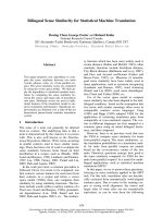
We first used the conditional cluster model of the
form P(w
i
|CW
i-2
j
CW
i-1
j
). Some sample settings of
parameters (j, t
w
) are shown in Figure 1. The
performance was consistently improved by
increasing the number of clusters j, except at the
smallest sizes. The word trigram model was
consistently the best model, except at the smallest

sizes, and even then was only marginally worse than
the conditional cluster models. This is not surprising
because the conditional cluster model always
discards information for predicting words.
We then used the predictive cluster model of the
form P(PW
i
l
|w
i-2
w
i-1
)×P(w
i
|w
i-2
w
i-1
PW
i
l
), where only
predicted words are clustered. Some sample settings
of the parameters (l, t
c
, t
w
) are shown in Figure 2. For
simplicity, we assumed t
c

=t
w
, meaning that the same
pruning threshold values were used for both
sub-models. It turns out that predictive cluster
models achieve the best perplexity results at about
2^6 or 2^8 clusters. The models consistently
outperform the baseline word trigram models.
We finally returned to the ACM of Equation (5),
where both conditional words and the predicted
word are clustered (with different numbers of
clusters), and which is referred to as the combined
cluster model below. In addition, we allow different
values of the threshold for different sub-models.
Therefore, we need to optimize the model parameter
set l, j, k, t
c
, t
w
.
Based on the pilot experiment results using
conditional and predictive cluster models, we tried
combined cluster models for values l
∈ [4, 10], j,
k
∈
[8, 16]. We also allow j, k=all. Rather than plot
all points of all models together, we show only the
outer envelope of the points. That is, if for a given
model type and a given point there is some other

point of the same type with both lower perplexity
and smaller size than the first point, then we do not
plot the first, worse point.
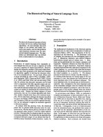
The results are shown in Figure 3, where the
cluster number of IBM models is 2^14 which
achieves the best performance for IBM models in
our experiments. It turns out that when l
∈ [6, 8] and
j, k>12, combined cluster models yield the best
results. We also found that the predictive cluster
models give as good performance as the best
combined ones while combined models
outperformed very slightly only when model sizes
are small. This is not difficult to explain. Recall that
the predictive cluster model is a special case of the
combined model where words are used in
conditional positions, i.e. j=k=all. Our experiments
show that combined models achieved good
performance when large numbers of clusters are
used for conditional words, i.e. large j, k>12, which
are similar to words.
The most interesting analysis is to look at some
sample settings of the parameters of the combined
cluster models in Figure 3. In Table 2, we show the
best parameter settings at several levels of model
size. Notice that in larger model sizes, predictive
cluster models (i.e. j=k=all) perform the best in
some cases. The ‘prune’ columns (i.e. columns 6 and
7) indicate the Stolcke pruning parameter we used.
First, notice that the two pruning parameters (in

columns 6 and 7) tend to be very similar. This is
desirable since applying the theory of relative
entropy pruning predicts that the two pruning
parameters should actually have the same value.
Next, let us compare the ACM
P(PW
i
l
|CW
i-2
j
CW
i-1
j
)×P(w
i
|CW
i-2
k
CW
i-1
k
PW
i
l
) to
traditional IBM clustering of the form
P(W
i
l

|W
i-2
l
W
i-1
l
)×P(w
i
|W
i
l
), which is equal to
P(W
i
l
|W
i-2
l
W
i-1
l
)×P(w
i
|W
i-2
0
W
i-1
0
W

i
l
) (assuming the
105
110
115
120
125
130
135
140
145
150
0.0E+00 5.0E+05 1.0E+06 1. 5E+06 2.0E+06 2.5E+06
size
perplexity
2^12 clusters
2^14 clusters
2^16 clusters
word trigram

Figure 1. Comparison of conditional models
applied with different numbers of clusters
100
105
110
115
120
125
130

135
140
145
150
0.0E+00 5.0E+05 1.0E+06 1.5E+06 2.0E+06 2.5E+06
size
perplexity
2^4 clusters
2^6 clusters
2^8 clusters
2^10 clusters
word trigram

Figure 2. Comparison of predictive models
applied with different numbers of clusters
100
110
120
130
140
150
160
170
0.0E+00 5.0E+05 1.0E+06 1.5E+06 2.0E+06 2.5E+06
size
perplexity
ACM
IBM
word trigram
predictive model

Figure 3. Comparison of ACMs, predictive
cluster model, IBM model, and word trigram
model
same type of cluster is used for both predictive and
conditional words). Our results in Figure 3 show that
the performance of IBM models is roughly an order
of magnitude worse than that of ACMs. This is
because in addition to the use of the symmetric
cluster model, the traditional IBM model makes two
more assumptions that we consider suboptimal.
First, it assumes that j=l. We see that the best results
come from unequal settings of j and l. Second, more
importantly, IBM clustering assumes that k=0. We
see that not only is the optimal setting for k not 0, but
also typically the exact opposite is the optimal: k=all
in which case P(w
i
|CW
i-2
k
CW
i-1
k
PW
i
l
)=
P(w
i

|w
i-2
w
i-1
PW
i
l
), or k=14, 16, which is very
similar. That is, we see that words depend on the
previous words and that an independence
assumption is a poor one. Of course, many of these
word dependencies are pruned away – but when a
word does depend on something, the previous words
are better predictors than the previous clusters.
Another important finding here is that for most of
these settings, the unpruned model is actually larger
than a normal trigram model – whenever k=all or 14,
16, the unpruned model P(PW
i
l
|CW
i-2
j
CW
i-1
j
) ×
P(w
i
|CW

i-2
k
CW
i-1
k
PW
i
l
) is actually larger than an
unpruned model P(w
i
|w
i-2
w
i-1
).
This analysis of the data is very interesting – it
implies that the gains from clustering are not from
compression, but rather from capturing structure.
Factoring the model into two models, in which the
cluster is predicted first, and then the word is
predicted given the cluster, allows the structure and
regularities of the model to be found. This larger,
better structured model can be pruned more
effectively, and it achieved better performance than
a word trigram model at the same model size.
Model size Perplexity l j k t
c
t
w

2.0E+05 141.1 8 12 14 24 24
2.5E+05 135.7 8 12 14 12 24
5.0E+05 118.8 6 14 16 6 12
7.5E+05 112.8 6 16 16 3 6
1.0E+06 109.0 6 16 16 3 3
1.3E+06 107.4 6 16 16 2 3
1.5E+06 106.0 6 All all 2 2
1.9E+06 104.9 6 All all 1 2
Table 2: Sample parameter settings for the ACM
4.5 CER results
Before we present CER results of the Japanese
Kana-Kanji conversion system, we briefly describe
our method for storing the ACM in practice.
One of the most common methods for storing
backoff n-gram models is to store n-gram
probabilities (and backoff weights) in a tree
structure, which begins with a hypothetical root
node that branches out into unigram nodes at the first
level of the tree, and each of those unigram nodes in
turn branches out into bigram nodes at the second
level and so on. To save storage, n-gram
probabilities such as P(w
i
|w
i-1
) and backoff weights
such as α(w
i-2
w

i-1
) are stored in a single (bigram)
node array (Clarkson and Rosenfeld, 1997).
Applying the above tree structure to storing the
ACM is a bit complicated – there are some
representation issues. For example, consider the
cluster sub-model P(PW
i
l
|CW
i-2
j
CW
i-1
j
). N-gram
probabilities such as P(PW
i
l
|CW
i-1
j
) and backoff
weights such as α(CW
i-2
j
CW
i-1
j
) cannot be stored in a

single (bigram) node array, because l ≠ j and
PW≠CW. Therefore, we used two separate trees to
store probabilities and backoff weights,
respectively. As a result, we used four tree structures
to store ACMs in practice: two for the cluster
sub-model P(PW
i
l
|CW
i-2
j
CW
i-1
j
), and two for the
word sub-model P(w
i
|CW
i-2
k
CW
i-1
k
PW
i
l
). We found
that the effect of the storage structure cannot be
ignored in a real application.
In addition, we used several techniques to

compress model parameters (i.e. word id, n-gram
probability, and backoff weight, etc.) and reduce the
storage space of models significantly. For example,
rather than store 4-byte floating point values for all
n-gram probabilities and backoff weights, the values
are quantized to a small number of quantization
levels. Quantization is performed separately on each
of the n-gram probability and backoff weight lists,
and separate quantization level look-up tables are
generated for each of these sets of parameters. We
used 8-bit quantization, which shows no
performance decline in our experiments.
Our goal is to achieve the best tradeoff between
performance and model size. Therefore, we would
like to compare the ACM with the word trigram
model at the same model size. Unfortunately, the
ACM contains four sub-models and this makes it
difficult to be pruned to a specific size. Thus for
comparison, we always choose the ACM with
smaller size than its competing word trigram model
to guarantee that our evaluation is under-estimated.
Experiments show that the ACMs achieve
statistically significant improvements over word
trigram models at even smaller model sizes (p-value
=8.0E-9). Some results are shown in Table 3.
Word trigram model ACM
Size
(MB)
CER Size
(MB)

CER CER
Reduction
1.8 4.56% 1.7 4.25% 6.8%
5.8 4.08% 4.5 3.83% 6.1%
11.7 4.04% 10.7 3.73% 7.7%
23.5 4.00% 21.7 3.63% 9.3%
42.4 3.98% 40.4 3.63% 8.8%
Table 3: CER results of ACMs and word
trigram models at different model sizes
Now we discuss why the ACM is superior to
simple word trigrams. In addition to the better
structure as shown in Section 3.3, we assume here
that the benefit of our model also comes from its
better smoothing. Consider a probability such as
P(Tuesday| party on). If we put the word “Tuesday”
into the cluster WEEKDAY, we decompose the
probability
When each word belongs to one class, simple math
shows that this decomposition is a strict equality.
However, when smoothing is taken into
consideration, using the clustered probability will be
more accurate than using the non-clustered
probability. For instance, even if we have never seen
an example of “party on Tuesday”, perhaps we have
seen examples of other phrases, such as “party on
Wednesday”; thus, the probability P(WEEKDAY |
party on) will be relatively high. Furthermore,
although we may never have seen an example of
“party on WEEKDAY Tuesday”, after we backoff or
interpolate with a lower order model, we may able to

accurately estimate P(Tuesday | on WEEKDAY).
Thus, our smoothed clustered estimate may be a
good one.
Our assumption can be tested empirically by
following experiments. We first constructed several
test sets with different backoff rates
4
. The backoff
rate of a test set, when presented to a trigram model,
is defined as the number of words whose trigram
probabilities are estimated by backoff bigram
probabilities divided by the number of words in the
test set. Then for each test set, we obtained a pair of
CER results using the ACM and the word trigram
model respectively. As shown in Figure 4, in both
cases, CER increases as the backoff rate increases
from 28% to 40%. But the curve of the word trigram
model has a steeper upward trend. The difference of
the upward trends of the two curves can be shown
more clearly by plotting the CER difference between
them, as shown in Figure 5. The results indicate that
because of its better smoothing, when the backoff
rate increases, the CER using the ACM does not
increase as fast as that using the word trigram model.
Therefore, we are reasonably confident that some
portion of the benefit of the ACM comes from its
better smoothing.
2.1
2.3
2.5

2.7
2.9
3.1
3.3
3.5
3.7
3.9
0.28 0.29 0.3 0.31 0.32 0.33 0.34 0.35 0.36 0.37 0.38 0.39 0.4 0.41
backoff rate
error rate
word trigram model
ACM

Figure 4: CER vs. backoff rate.


4
The backoff rates are estimated using the baseline
trigram model, so the choice could be biased against the
word trigram model.
P(Tuesday | party on) = P(WEEKDAY | party on)
×

P(Tuesday | party on WEEKDAY).
0.25
0.27
0.29
0.31
0.33
0.35

0.37
0.39
0.41
0.28 0.3 0.32 0.34 0.36 0.38 0.4 0.42
backoff rate
error rate difference

Figure 5: CER difference vs. backoff rate.
5 Conclusion
There are three main contributions of this paper.
First, after presenting a formal definition of the
ACM, we described in detail the methodology of
constructing the ACM effectively. We showed
empirically that both the asymmetric clustering and
the parameter optimization (i.e. optimal cluster
numbers) have positive impacts on the performance
of the resulting ACM. The finding demonstrates
partially the effectiveness of our research focus:
techniques for using clusters (i.e. the ACM) rather
than techniques for finding clusters (i.e. clustering
algorithms). Second, we explored the actual
representation of the ACM and evaluate it on a
realistic application – Japanese Kana-Kanji
conversion. Results show approximately 6-10%
CER reduction of the ACMs in comparison with the
word trigram models, even when the ACMs are
slightly smaller. Third, the reasons underlying the
superiority of the ACM are analyzed. For instance,
our analysis suggests the benefit of the ACM comes
partially from its better structure and its better

smoothing.
All cluster models discussed in this paper are
based on hard clustering, meaning that each word
belongs to only one cluster. One area we have not
explored is the use of soft clustering, where a word w
can be assigned to multiple clusters W with a
probability P(W|w) [Pereira et al., 1993]. Saul and
Pereira [1997] demonstrated the utility of soft
clustering and concluded that any method that
assigns each word to a single cluster would lose
information. It is an interesting question whether our
techniques for hard clustering can be extended to
soft clustering. On the other hand, soft clustering
models tend to be larger than hard clustering models
because a given word can belong to multiple
clusters, and thus a training instance P(w
i
|w
i-2
w
i-1
)
can lead to multiple counts instead of just 1.
References
Bai, S., Li, H., Lin, Z., and Yuan, B. (1998). Building
class-based language models with contextual statistics. In
ICASSP-98, pp. 173-176.
Bellegarda, J. R., Butzberger, J. W., Chow, Y. L., Coccaro, N.
B., and Naik, D. (1996). A novel word clustering algorithm
based on latent semantic analysis. In ICASSP-96.

Brown, P. F., Cocke, J., DellaPietra, S. A., DellaPietra, V. J.,
Jelinek, F., Lafferty, J. D., Mercer, R. L., and Roossin, P. S.
(1990). A statistical approach to machine translation.
Computational Linguistics, 16(2), pp. 79-85.
Brown, P. F., DellaPietra V. J., deSouza, P. V., Lai, J. C., and
Mercer, R. L. (1992). Class-based n-gram models of natural
language. Computational Linguistics, 18(4), pp. 467-479.
Clarkson, P. R., and Rosenfeld, R. (1997). Statistical language
modeling using the CMU-Cambridge toolkit. In Eurospeech
1997, Rhodes, Greece.
Gao, J. Goodman, J. and Miao, J. (2001). The use of clustering
techniques for language model – application to Asian
language. Computational Linguistics and Chinese Language
Processing. Vol. 6, No. 1, pp 27-60.
Gao, J., Goodman, J., Li, M., and Lee, K. F. (2002). Toward a
unified approach to statistical language modeling for Chinese.
ACM Transactions on Asian Language Information
Processing. Vol. 1, No. 1, pp 3-33.
Goodman, J. (2001). A bit of progress in language modeling. In
Computer Speech and Language, October 2001, pp 403-434.
Goodman, J., and Gao, J. (2000). Language model size
reduction by predictive clustering. ICSLP-2000, Beijing.
Jelinek, F. (1990). Self-organized language modeling for speech
recognition. In Readings in Speech Recognition, A. Waibel
and K. F. Lee, eds., Morgan-Kaufmann, San Mateo, CA, pp.
450-506.
Katz, S. M. (1987). Estimation of probabilities from sparse data
for the language model component of a speech recognizer.
IEEE Transactions on Acoustics, Speech and Signal
Processing, ASSP-35(3):400-401, March.

Kneser, R. and Ney, H. (1993). Improved clustering techniques
for class-based statistical language modeling. In Eurospeech,
Vol. 2, pp. 973-976, Berlin, Germany.
Ney, H., Essen, U., and Kneser, R. (1994). On structuring
probabilistic dependences in stochastic language modeling.
Computer, Speech, and Language, 8:1-38.
Pereira, F., Tishby, N., and Lee L. (1993). Distributional
clustering of English words. In Proceedings of the 31
st
Annual
Meeting of the ACL.
Rosenfeld, R. (2000). Two decades of statistical language
modeling: where do we go from here. In Proceeding of the
IEEE, 88:1270-1278, August.
Saul, L., and Pereira, F.C.N. (1997). Aggregate and mixed-order
Markov models for statistical language processing. In
EMNLP-1997.
Stolcke, A. (1998). Entropy-based Pruning of Backoff
Language Models. Proc. DARPA News Transcription and
Understanding Workshop, 1998, pp. 270-274.
Ueberla, J. P. (1996). An extended clustering algorithm for
statistical language models. IEEE Transactions on Speech
and Audio Processing, 4(4): 313-316.
Yamamoto, H., Isogai, S., and Sagisaka, Y. (2001). Multi-Class
Composite N-gram Language Model for Spoken Language
Processing Using Multiple Word Clusters. 39
th
Annual
meetings of the Association for Computational Linguistics
(ACL’01), Toulouse, 6-11 July 2001.

Yamamoto, H., and Sagisaka, Y. (1999). Multi-class Composite
N-gram based on Connection Direction, In Proceedings of the
IEEE International Conference on Acoustics, Speech and
Signal Processing, May, Phoenix, Arizona.