Báo cáo khoa học: " New Ranking Algorithms for Parsing and Tagging: Kernels over Discrete Structures, and the Voted Perceptron" docx
Bạn đang xem bản rút gọn của tài liệu. Xem và tải ngay bản đầy đủ của tài liệu tại đây (100.58 KB, 8 trang )
New Ranking Algorithms for Parsing and Tagging:
Kernels over Discrete Structures, and the Voted Perceptron
Michael Collins
AT&T Labs-Research,
Florham Park,
New Jersey.
Nigel Duffy
iKuni Inc.,
3400 Hillview Ave., Building 5,
Palo Alto, CA 94304.
Abstract
This paper introduces new learning al-
gorithms for natural language processing
based on the perceptron algorithm. We
show how the algorithms can be efficiently
applied to exponential sized representa-
tions of parse trees, such as the “all sub-
trees” (DOP) representation described by
(Bod 1998), or a representation tracking
all sub-fragments of a tagged sentence.
We give experimental results showing sig-
nificant improvements on two tasks: pars-
ing Wall Street Journal text, and named-
entity extraction from web data.
1 Introduction
The perceptron algorithm is one of the oldest algo-
rithms in machine learning, going back to (Rosen-
blatt 1958). It is an incredibly simple algorithm to
implement, and yet it has been shown to be com-
petitive with more recent learning methods such as
support vector machines – see (Freund & Schapire
1999) for its application to image classification, for
example.
This paper describes how the perceptron and
voted perceptron algorithms can be used for pars-
ing and tagging problems. Crucially, the algorithms
can be efficiently applied to exponential sized repre-
sentations of parse trees, such as the “all subtrees”
(DOP) representation described by (Bod 1998), or a
representation tracking all sub-fragments of a tagged
sentence. It might seem paradoxical to be able to ef-
ficiently learn and apply amodel with an exponential
number of features.
1
The key to our algorithms is the
1
Although see (Goodman 1996) for an efficient algorithm
for the DOP model, which we discuss in section 7 of this paper.
“kernel” trick ((Cristianini and Shawe-Taylor 2000)
discuss kernel methods at length). We describe how
the inner product between feature vectors in these
representations can be calculated efficiently using
dynamic programming algorithms. This leads to
polynomial time
2
algorithms for training and apply-
ing the perceptron. The kernels we describe are re-
lated to the kernels over discrete structures in (Haus-
sler 1999; Lodhi et al. 2001).
A previous paper (Collins and Duffy 2001)
showed improvements over a PCFG in parsing the
ATIS task. In this paper we show that the method
scales to far more complex domains. In parsing Wall
Street Journal text, the method gives a 5.1% relative
reduction in error rate over the model of (Collins
1999). In the second domain, detecting named-
entity boundaries in web data, we show a 15.6% rel-
ative error reduction (an improvement in F-measure
from 85.3% to 87.6%) over a state-of-the-art model,
a maximum-entropy tagger. This result is derived
using a new kernel, for tagged sequences, described
in this paper. Both results rely on a new approach
that incorporates the log-probability from a baseline
model, in addition to the “all-fragments” features.
2 Feature–Vector Representations of Parse
Trees and Tagged Sequences
This paper focuses on the task of choosing the cor-
rect parse or tag sequence for a sentence from a
group of “candidates” for that sentence. The candi-
dates might be enumerated by a number of methods.
The experiments in this paper use the top
candi-
dates from a baseline probabilistic model: the model
of (Collins 1999) for parsing, and a maximum-
entropy tagger for named-entity recognition.
2
i.e., polynomial in the number of training examples, and
the size of trees or sentences in training and test data.
Computational Linguistics (ACL), Philadelphia, July 2002, pp. 263-270.
Proceedings of the 40th Annual Meeting of the Association for
The choice of representation is central: what fea-
tures should be used as evidence in choosing be-
tween candidates? We will use a function
to denote a -dimensional feature vector that rep-
resents a tree or tagged sequence
. There are many
possibilities for . An obvious example for parse
trees is to have one component of for each
rule in a context-free grammar that underlies the
trees. This is the representation used by Stochastic
Context-Free Grammars. The feature vector tracks
the counts of rules in the tree , thus encoding the
sufficient statistics for the SCFG.
Given a representation, and two structures and
, the inner product between the structures can be
defined as
The idea of inner products between feature vectors
is central to learning algorithms such as Support
Vector Machines (SVMs), and is also central to the
ideas in this paper. Intuitively, the inner product
is a similarity measure between objects: structures
with similar feature vectors will have high values for
. More formally, it has been observed that
many algorithms can be implemented using inner
products between training examples alone, without
direct access to the feature vectors themselves. As
we will see in this paper, this can be crucial for the
efficiency of learning with certain representations.
Following the SVM literature, we call a function
of two objects and a “kernel” if it can
be shown that is an inner product in some feature
space .
3 Algorithms
3.1 Notation
This section formalizes the idea of linear models for
parsing or tagging. The method is related to the
boosting approach to ranking problems (Freund et
al. 1998), the Markov Random Field methods of
(Johnson et al. 1999), and the boosting approaches
for parsing in (Collins 2000). The set-up is as fol-
lows:
Training data is a set of example input/output
pairs. In parsing the training examples are
where each is a sentence and each is the correct
tree for that sentence.
We assume some way of enumerating a set of
candidates for a particular sentence. We use to
denote the
’th candidate for the ’th sentence in
training data, and to denote
the set of candidates for .
Without loss of generality we take to be the
correct candidate for (i.e., ).
Each candidate is represented by a feature
vector in the space . The parameters of
the model are also a vector . The out-
put of the model on a training or test example is
.
The key question, having defined a representation
, is how to set the parameters . We discuss one
method for setting the weights, the perceptron algo-
rithm, in the next section.
3.2 The Perceptron Algorithm
Figure 1(a) shows the perceptron algorithm applied
to the ranking task. The method assumes a training
set as described in section 3.1, and a representation
of parse trees. The algorithm maintains a param-
eter vector
, which is initially set to be all zeros.
The algorithm then makes a pass over the training
set, only updating the parameter vector when a mis-
take is made on an example. The parameter vec-
tor update is very simple, involving adding the dif-
ference of the offending examples’ representations
(
in the figure). Intu-
itively, this update has the effect of increasing the
parameter values for features in the correct tree, and
downweighting the parameter values for features in
the competitor.
See (Cristianini and Shawe-Taylor 2000) for dis-
cussion of the perceptron algorithm, including an
overview of various theorems justifying this way of
setting the parameters. Briefly, the perceptron algo-
rithm is guaranteed
3
to find a hyperplane that cor-
rectly classifies all training points, if such a hyper-
plane exists (i.e., the data is “separable”). Moreover,
the number of mistakes made will be low, providing
that the data is separable with “large margin”, and
3
To find such a hyperplane the algorithm must be run over
the training set repeatedly until no mistakes are made. The al-
gorithm in figure 1 includes just a single pass over the training
set.
(a) Define: (b)Define:
.
Initialization: Set parameters Initialization: Set dual parameters
For For
If Then If Then
Output on test sentence : Output on test sentence :
.
Figure 1: a) The perceptron algorithm for ranking problems. b) The algorithm in dual form.
this translates to guarantees about how the method
generalizes to test examples. (Freund & Schapire
1999) give theorems showing that the voted per-
ceptron (a variant described below) generalizes well
even given non-separable data.
3.3 The Algorithm in Dual Form
Figure 1(b) shows an equivalent algorithm to the
perceptron, an algorithm which we will call the
“dual form” of the perceptron. The dual-form al-
gorithm does not store a parameter vector , in-
stead storing a set of dual parameters, for
. The score for a parse is de-
fined by the dual parameters as
This is in contrast to , the score in
the original algorithm.
In spite of these differences the algorithms
give identical results on training and test exam-
ples: to see this, it can be verified that
, and hence that
, throughout training.
The important difference between the algorithms
lies in the analysis of their computational complex-
ity. Say is the size of the training set, i.e.,
. Also, take to be the dimensional-
ity of the parameter vector . Then the algorithm
in figure 1(a) takes time.
4
This follows be-
cause must be calculated for each member of
the training set, and each calculation of involves
time. Now say the time taken to compute the
4
If the vectors are sparse, then can be taken to be the
number of non-zero elements of , assuming that it takes
time to add feature vectors with non-zero elements, or to
take inner products.
inner product between two examples is . The run-
ning time of the algorithm in figure 1(b) is .
This follows because throughout the algorithm the
number of non-zero dual parameters is bounded by
, and hence the calculation of takes at most
time. (Note that the dual form algorithm runs
in quadratic time in the number of training examples
, because .)
The dual algorithm is therefore more efficient in
cases where
. This might seem unlikely to
be the case – naively, it would be expected that the
time to calculate the inner product
be-
tween two vectors to be at least . But it turns
out that for some high-dimensional representations
the inner product can be calculated in much bet-
ter than
time, making the dual form algorithm
more efficient than the original algorithm. The dual-
form algorithm goes back to (Aizerman et al. 64).
See (Cristianini and Shawe-Taylor 2000) for more
explanation of the algorithm.
3.4 The Voted Perceptron
(Freund & Schapire 1999) describe a refinement of
the perceptron algorithm, the “voted perceptron”.
They give theory which suggests that the voted per-
ceptron is preferable in cases of noisy or unsepara-
ble data. The training phase of the algorithm is un-
changed – the change isin how the method is applied
to test examples. The algorithm in figure 1(b) can be
considered to build a series of hypotheses
, for
, where is defined as
is the scoring function from the algorithm trained
on just the first training examples. The output of a
model trained on the first examples for a sentence
a) S
NP
N
John
VP
V
saw
NP
D
the
N
man
b) NP
D
the
N
man
NP
D N
D
the
N
man
NP
D
the
N
NP
D N
man
Figure 2: a) An example parsetree. b) The sub-trees of the NP
covering the man. The tree in (a) contains all of these subtrees,
as well as many others.
is . Thus the training
algorithm can be considered to construct a sequence
of
models, . On a test sentence , each
of these functions will return its own parse tree,
for . The voted perceptron picks
the most likely tree as that which occurs most often
in the set .
Note that is easily derived from ,
through the identity
. Be-
cause of this the voted perceptron can be imple-
mented with the same number of kernel calculations,
and henceroughly the same computational complex-
ity, as the original perceptron.
4 A Tree Kernel
We now consider a representation that tracks all sub-
trees seen in training data, the representation stud-
ied extensively by (Bod 1998). See figure 2 for
an example. Conceptually we begin by enumer-
ating all tree fragments that occur in the training
data
. Note that this is done only implicitly.
Each tree is represented by a dimensional vector
where the ’th component counts the number of oc-
curences of the ’th tree fragment. Define the func-
tion to be the number of occurences of the ’th
tree fragment in tree , so that is now represented
as . Note that
will be huge (a given tree will have a number of sub-
trees that is exponential in its size). Because of this
we aim to design algorithms whose computational
complexity is independent of .
The key to our efficient use of this representa-
tion is a dynamic programming algorithm that com-
putes the inner product between two examples
and in polynomial (in the size of the trees in-
volved), rather than
, time. The algorithm is
described in (Collins and Duffy 2001), but for com-
pleteness we repeat it here. We first define the set
of nodes in trees and as and respec-
tively. We define the indicator function to be
if sub-tree is seen rooted at node and 0 other-
wise. It follows that and
. The first step to efficient
computation of the inner product is the following
property:
where we define .
Next, we note that can be computed ef-
ficiently, due to the following recursive definition:
If the productions at and are different
.
If the productions at and are the same, and
and are pre-terminals, then .
5
Else if the productions at and are the same
and and are not pre-terminals,
where is the number of children of in the
tree; because the productions at / are the same,
we have . The ’th child-node of
is .
To see that this recursive definition is correct, note
that simply counts
the number of common subtrees that are found
rooted at both and . The first two cases are
trivially correct. The last, recursive, definition fol-
lows because a common subtree for and can
be formed by taking the production at / , to-
gether with a choice at each child of simply tak-
ing the non-terminal at that child, or any one of
the common sub-trees at that child. Thus there are
5
Pre-terminals are nodes directly above words in the surface
string, for example the N, V, and D symbols in Figure 2.
Lou Gerstner is chairman of IBM
N N V N P N
N V
Gerstner is
NN
Lou
N
Lou
N V
a)
b)
Figure 3: a) A tagged sequence. b) Example “fragments”
of the tagged sequence: the tagging kernel is sensitive to the
counts of all such fragments.
possible choices
at the ’th child. (Note that a similar recursion is de-
scribed by Goodman (Goodman 1996), Goodman’s
application being the conversion of Bod’s model
(Bod 1998) to an equivalent PCFG.)
It is clear from the identity
, and the recursive definition of
, that can be calculated in
time: the matrix of values
can be filled in, then summed.
6
Since there will be many more tree fragments
of larger size – say depth four versus depth three
– it makes sense to downweight the contribu-
tion of larger tree fragments to the kernel. This
can be achieved by introducing a parameter
, and modifying the base case and re-
cursive case of the definitions of to be re-
spectively and
. This cor-
responds to a modified kernel
where is the number of
rules in the ’th fragment. This is roughly equiva-
lent to having a prior that large sub-trees will be less
useful in the learning task.
5 A Tagging Kernel
The second problem we consider is tagging, where
each word in a sentence is mapped to one of a finite
set of tags. The tags might represent part-of-speech
tags, named-entity boundaries, base noun-phrases,
or other structures. In the experiments in this paper
we consider named-entity recognition.
6
This can be a pessimistic estimate of the runtime. A more
useful characterization is that it runs intime linear in the number
of members such that the productions at
and are the same. In our data we have found the number
of nodes with identical productions to be approximately linear
in the size of the trees, so the running time is also close to linear
in the size of the trees.
A tagged sequence is a sequence of word/state
pairs where is the ’th
word, and is the tag for that word. The par-
ticular representation we consider is similar to the
all sub-trees representation for trees. A tagged-
sequence “fragment” is a subgraph that contains a
subsequence of state labels, where each label may
or may not contain the word below it. See figure 3
for anexample. Each tagged sequence is represented
by a
dimensional vector where the ’th component
counts the number of occurrences of the ’th
fragment in .
The inner product under this representation can
be calculated using dynamic programming in a very
similar way to the tree algorithm. We first define
the set of states in tagged sequences and as
and respectively. Each state has an asso-
ciated label and an associated word. We define
the indicator function to be if fragment
is seen with left-most state at node , and 0 other-
wise. It follows that and
. As before, some simple
algebra shows that
where we define .
Next, for any given state define
to be the state to the right of in the structure
. An analogous definition holds for .
Then can be computed using dynamic
programming, due to a recursive definition:
If the state labels at and are different
.
If the state labels at and are the same,
but the words at and are different, then
.
Else if the state labels at and are the
same, and the words at and are the same, then
.
There are a couple of useful modifications to this
kernel. One is to introduce a parameter
which penalizes larger substructures. The recur-
sive definitions are modfied to be
and
respectively. This gives
an inner product where
is the number of state labels in the th fragment.
Another useful modification is as follows. Define
MODEL 40 Words (2245 sentences)
LR LP CBs CBs CBs
CO99 88.5% 88.7% 0.92 66.7% 87.1%
VP 89.1% 89.4% 0.85 69.3% 88.2%
MODEL 100 Words (2416 sentences)
LR LP CBs CBs CBs
CO99 88.1% 88.3% 1.06 64.0% 85.1%
VP 88.6% 88.9% 0.99 66.5% 86.3%
Figure 4: Results on Section 23 of the WSJ Treebank. LR/LP
= labeled recall/precision. CBs = average number of crossing
brackets per sentence. 0 CBs,
CBs are the percentage of sen-
tences with 0 or crossing brackets respectively. CO99 is
model 2 of (Collins 1999). VP is the voted perceptron with the
tree kernel.
for words and to be if
, otherwise. Define to be if
and share the same word features, 0 otherwise.
For example,
might be defined to be 1 if
and are both capitalized: in this case is
a looser notion of similarity than the exact match
criterion of . Finally, the definition of can
be modified to:
If labels at are different, .
Else
where , are the words at and respec-
tively. This inner product implicitly includes fea-
tures which track word features, and thus can make
better use of sparse data.
6 Experiments
6.1 Parsing Wall Street Journal Text
We used the same data set as that described in
(Collins 2000). The Penn Wall Street Journal tree-
bank (Marcus et al. 1993) was used as training and
test data. Sections 2-21 inclusive (around 40,000
sentences) were used as training data, section 23
was used as the final test set. Of the 40,000 train-
ing sentences, the first 36,000 were used to train
the perceptron. The remaining 4,000 sentences were
used as development data, and for tuning parame-
ters of the algorithm. Model 2 of (Collins 1999) was
used to parse both the training and test data, produc-
ing multiple hypotheses for each sentence. In or-
der to gain a representative set of training data, the
36,000 training sentences were parsed in 2,000 sen-
tence chunks, each chunk being parsed with a model
trained on the remaining 34,000 sentences (this pre-
vented the initial model from being unrealistically
“good” on the training sentences). The 4,000 devel-
opment sentences were parsed with a model trained
on the 36,000 training sentences. Section 23 was
parsed with a model trained on all 40,000 sentences.
The representation we use incorporates the prob-
ability from the original model, as well as the
all-subtrees representation. We introduce a pa-
rameter
which controls the relative contribu-
tion of the two terms. If is the log prob-
ability of a tree under the original probability
model, and is
the feature vector under the all subtrees represen-
tation, then the new representation is
, and the inner
product between two examples and is
. This allows the
perceptron algorithm to use the probability from the
original model as well as the subtrees information to
rank trees. We would thus expect the model to do at
least as well as the original probabilistic model.
The algorithm in figure 1(b) was applied to the
problem, with the inner product
used
in the definition of . The algorithm in 1(b)
runs in approximately quadratic time in the number
of training examples. This made it somewhat ex-
pensive to run the algorithm over all 36,000 training
sentences in one pass. Instead, we broke the training
set into 6 chunks of roughly equal size, and trained
6 separate perceptrons on these data sets. This has
the advantage of reducing training time, both be-
cause of the quadratic dependence on training set
size, and also because it is easy to train the 6 models
in parallel. The outputs from the 6 runs on test ex-
amples were combined through the voting procedure
described in section 3.4.
Figure 4 shows the results for the voted percep-
tron with the tree kernel. The parameters
and
were set to and respectively through tun-
ing on the development set. The method shows
a absolute improvement in average preci-
sion and recall (from 88.2% to 88.8% on sentences
words), a 5.1% relative reduction in er-
ror. The boosting method of (Collins 2000) showed
89.6%/89.9% recall and precision on reranking ap-
proaches for the same datasets (sentences less than
100 words in length). (Charniak 2000) describes a
different method which achieves very similar per-
formance to (Collins 2000). (Bod 2001) describes
experiments giving 90.6%/90.8% recall and preci-
sion for sentences of less than 40 words in length,
using the all-subtrees representation, but using very
different algorithms and parameter estimation meth-
ods from the perceptron algorithms in this paper (see
section 7 for more discussion).
6.2 Named–Entity Extraction
Over a period of a year or so we have had over one
million words of named-entity data annotated. The
data is drawn from web pages, the aim being to sup-
port a question-answering system over web data. A
number of categories are annotated: the usual peo-
ple, organization and location categories, as well as
less frequent categories such as brand-names, scien-
tific terms, event titles (such as concerts) and so on.
As a result, we created a training set of 53,609 sen-
tences (1,047,491 words), and a test set of 14,717
sentences (291,898 words).
The task we consider is to recover named-entity
boundaries. We leave the recovery of the categories
of entities to a separate stage of processing. We eval-
uate different methods on the task through precision
and recall.
7
The problem can be framed as a tag-
ging task – to tag each word as being either the start
of an entity, a continuation of an entity, or not to
be part of an entity at all. As a baseline model we
used a maximum entropy tagger, very similar to the
one described in (Ratnaparkhi 1996). Maximum en-
tropy taggers have been shown to be highly com-
petitive on a number of tagging tasks, such as part-
of-speech tagging (Ratnaparkhi 1996), and named-
entity recognition (Borthwick et. al 1998). Thus
the maximum-entropy tagger we used represents a
serious baseline for the task. We used a feature
set which included the current, next, and previous
word; the previous two tags; various capitalization
and other features of the word being tagged (the full
feature set is described in (Collins 2002a)).
As a baseline we trained a model on the full
53,609 sentences of training data, and decoded the
14,717 sentences of test data using a beam search
7
If a method proposes entities on the test set, and of
these are correct then the precision of a method is .
Similarly, if is the number of entities in the human annotated
version of the test set, then the recall is .
P R F
Max-Ent 84.4% 86.3% 85.3%
Perc. 86.1% 89.1% 87.6%
Imp. 10.9% 20.4% 15.6%
Figure 5: Results for the max-ent and voted perceptron meth-
ods. “Imp.” is the relative error reduction given by using the
perceptron.
precision, recall, F-measure.
which keeps the top 20 hypotheses at each stage of
a left-to-right search. In training the voted percep-
tron we split the training data into a 41,992 sen-
tence training set, and a 11,617 sentence develop-
ment set. The training set was split into 5 portions,
and in each case the maximum-entropy tagger was
trained on 4/5 of the data, then used to decode the
remaining 1/5. In this way the whole training data
was decoded. The top 20 hypotheses under a beam
search, together with their log probabilities, were re-
covered for each training sentence. In a similar way,
a model trained on the 41,992 sentence set was used
to produce 20 hypotheses for each sentence in the
development set.
As in the parsing experiments, the final kernel in-
corporates the probability from the maximum en-
tropy tagger, i.e.
where is the log-likelihood of
under the tagging model, is the tagging
kernel described previously, and
is a parameter
weighting the two terms. The other free parame-
ter in the kernel is
, which determines how quickly
larger structures are downweighted. In running sev-
eral training runs with different parameter values,
and then testing error rates on the development set,
the best parameter values we found were
,
. Figure 5 shows results on the test data
for the baseline maximum-entropy tagger, and the
voted perceptron. The results show a 15.6% relative
improvement in F-measure.
7 Relationship to Previous Work
(Bod 1998) describes quite different parameter esti-
mation and parsing methods for the DOP represen-
tation. The methods explicitly deal with the param-
eters associated with subtrees, with sub-sampling of
tree fragments making the computation manageable.
Even after this, Bod’s method is left with a huge
grammar: (Bod 2001) describes a grammar with
over 5 million sub-structures. The method requires
search for the 1,000 most probable derivations un-
der this grammar, using beam search, presumably a
challenging computational task given the size of the
grammar. In spite of these problems, (Bod 2001)
gives excellent results for the method on parsing
Wall Street Journal text. The algorithms in this paper
have a different flavor, avoiding the need to explic-
itly deal with feature vectors that track all subtrees,
and also avoiding the need to sum over an exponen-
tial number of derivations underlying a given tree.
(Goodman 1996) gives a polynomial time con-
version of a DOP model into an equivalent PCFG
whose size is linear in the size of the training set.
The method uses a similar recursion to the common
sub-trees recursion described in this paper. Good-
man’s method still leaves exact parsing under the
model intractable (because of the need to sum over
multiple derivations underlying the same tree), but
he gives an approximation to finding the most prob-
able tree, which can be computed efficiently.
From a theoretical point of view, it is difficult to
find motivation for the parameter estimation meth-
ods used by (Bod 1998) – see (Johnson 2002) for
discussion. In contrast, the parameter estimation
methods in this paper have a strong theoretical basis
(see (Cristianini and Shawe-Taylor 2000) chapter 2
and (Freund & Schapire 1999) for statistical theory
underlying the perceptron).
For related work on the voted perceptron algo-
rithm applied to NLP problems, see (Collins 2002a)
and (Collins 2002b). (Collins 2002a) describes ex-
periments on the same named-entity dataset as in
this paper, but using explicit features rather than ker-
nels. (Collins 2002b) describes how the voted per-
ceptron can be used to train maximum-entropy style
taggers, and also gives a more thorough discussion
of the theory behind the perceptron algorithm ap-
plied to ranking tasks.
Acknowledgements Many thanksto Jack Minisi for
annotating the named-entity data used in the exper-
iments. Thanks to Rob Schapire and Yoram Singer
for many useful discussions.
References
Aizerman, M., Braverman, E., & Rozonoer, L. (1964). Theoret-
ical Foundations of the Potential Function Method in Pattern
Recognition Learning. In Automation and Remote Control,
25:821–837.
Bod, R. (1998). Beyond Grammar: An Experience-Based The-
ory of Language. CSLI Publications/Cambridge University
Press.
Bod, R. (2001). What is the Minimal Set of Fragments that
Achieves Maximal Parse Accuracy? In Proceedings of ACL
2001.
Borthwick, A., Sterling, J., Agichtein, E., and Grishman, R.
(1998). Exploiting Diverse Knowledge Sources via Maxi-
mum Entropy in Named Entity Recognition. Proc. of the
Sixth Workshop on Very Large Corpora.
Charniak, E. (2000). A maximum-entropy-inspired parser. In
Proceedings of NAACL 2000.
Collins, M. 1999. Head-Driven Statistical Models for Natural
Language Parsing. PhD Dissertation, University of Pennsyl-
vania.
Collins, M. (2000). Discriminative Reranking for Natural Lan-
guage Parsing. Proceedings of the Seventeenth International
Conference on Machine Learning (ICML 2000).
Collins, M., and Duffy, N. (2001). Convolution Kernels for Nat-
ural Language. In Proceedings of Neural Information Pro-
cessing Systems (NIPS 14).
Collins, M. (2002a). Ranking Algorithms for Named–Entity
Extraction: Boosting and the Voted Perceptron. In Proceed-
ings of ACL 2002.
Collins, M. (2002b). Discriminative Training Methods for Hid-
den Markov Models: Theory and Experiments with the Per-
ceptron Algorithm. In Proceedings of EMNLP 2002.
Cristianini, N., and Shawe-Tayor, J. (2000). An introduction to
Support Vector Machines and other kernel-based learning
methods. Cambridge University Press.
Freund, Y. & Schapire, R. (1999). Large Margin Classifica-
tion using the Perceptron Algorithm. In Machine Learning,
37(3):277–296.
Freund, Y., Iyer, R.,Schapire, R.E., & Singer, Y. (1998). An effi-
cient boosting algorithm for combining preferences. In Ma-
chine Learning: Proceedings of the Fifteenth International
Conference. San Francisco: Morgan Kaufmann.
Goodman, J. (1996). Efficient algorithms for parsing the DOP
model. In Proceedings of the Conference on Empirical Meth-
ods in Natural Language Processing, pages 143-152.
Haussler, D. (1999). Convolution Kernels on Discrete Struc-
tures. Technical report, University of Santa Cruz.
Johnson, M., Geman, S., Canon, S., Chi, S., & Riezler, S.
(1999). Estimators for stochastic ‘unification-based” gram-
mars. In Proceedings of the 37th Annual Meeting of the As-
sociation for Computational Linguistics.
Johnson, M. (2002). The DOP estimation method is biased and
inconsistent. Computational Linguistics, 28, 71-76.
Lodhi, H., Christianini, N., Shawe-Taylor, J., & Watkins, C.
(2001). Text Classification using String Kernels. In Advances
in Neural Information Processing Systems 13, MIT Press.
Marcus, M., Santorini, B., & Marcinkiewicz, M. (1993). Build-
ing a large annotated corpus of english: The Penn treebank.
Computational Linguistics, 19, 313-330.
Ratnaparkhi, A. (1996). A maximum entropy part-of-speech
tagger. In Proceedings of the empirical methods in natural
language processing conference.
Rosenblatt, F. 1958. The Perceptron: A Probabilistic Model for
Information Storage and Organization in the Brain. Psycho-
logical Review, 65, 386–408. (Reprinted in Neurocomputing
(MIT Press, 1998).)