Báo cáo khoa học: "Word-Sense Disambiguation Using Decomposable Models and Janyce Wiebe" pdf

Word-Sense
Disambiguation Using Decomposable Models
Rebecca
Bruce and Janyce
Wiebe
Computing Research Lab
and
Department of Computer Science
New Mexico State University
Las Cruces, NM 88003
,
Abstract
Most probabilistic classifiers used for word-sense disam-
biguation have either been based on only one contextual
feature or have used a model that is simply assumed
to characterize the interdependencies among multiple
contextual features. In this paper, a different approach
to formulating a probabilistic model is presented along
with a case study of the performance of models pro-
duced in this manner for the disambiguation of the noun
interest. We describe a method for formulating proba-
bilistic models that use multiple contextual features for
word-sense disambiguation, without requiring untested
assumptions regarding the form of the model. Using
this approach, the joint distribution of all variables is
described by only the most systematic variable inter-
actions, thereby limiting the number of parameters to
be estimated, supporting computational efficiency, and
providing an understanding of the data.
Introduction
This paper presents a method for constructing prob-

abilistic classifiers for word-sense disambiguation that
offers advantages over previous approaches. Most pre-
vious efforts have not attempted to systematically iden-
tify the interdependencies among contextual features
(such as collocations) that can be used to classify the
meaning of an ambiguous word. Many researchers have
performed disambiguation on the basis of only a single
feature, while others who do consider multiple contex-
tual features assume that all contextual features are
either conditionally independent given the sense of the
word or fully independent. Of course, all contextual fea-
tures could be treated as interdependent, but, if there
are several features, such a model could have too many
parameters to estimate in practice.
We present a method for formulating probabilistic
models that describe the relationships among all vari-
ables in terms of only the most important interdepen-
dencies, that is, models of a certain class that are good
approximations to the joint distribution of contextual
features and word meanings. This class is the set of de-
composable models: models that can be expressed as a
product of marginal distributions, where each marginal
is composed of interdependent variables. The test used
to evaluate a model gives preference to those that have
the fewest number of interdependencies, thereby select-
ing models expressing only the most systematic variable
interactions.
To summarize the method, one first identifies infor-
mative contextual features (where "informative" is a
well-defined notion, discussed in Section 2). Then, out

of all possible decomposable models characterizing in-
terdependency relationships among the selected vari-
ables, those that are found to produce good approxima-
tions to the data are identified (using the test mentioned
above) and one of those models is used to perform dis-
ambiguation. Thus, we are able to use multiple contex-
tual features without the need for untested assumptions
regarding the form of the model. Further, approximat-
ing the joint distribution of all variables with a model
identifying only the most important systematic interac-
tions among variables limits the number of parameters
to be estimated, supports computational efficiency, and
provides an understanding of the data. The biggest lim-
itation associated with this method is the need for large
amounts of sense-tagged data. Because asymptotic dis-
tributions of the test statistics are used, the validity of
the results obtained using this approach are compro-
mised when it is applied to sparse data (this point is
discussed further in Section 2).
To test the method of model selection presented in
this paper, a case study of the disambiguation of the
noun interest was performed. Interest was selected be-
cause it has been shown in previous studies to be a dif-
ficult word to disambiguate. We selected as the set of
sense tags all non-idiomatic noun senses of interest de-
fined in the electronic version of Longman's Dictionary
of Contemporary English (LDOCE) ([23]). Using the
models produced in this study, we are able to assign an
LDOCE sense tag to every usage of interest in a held-
out test set with 78% accuracy. Although it is difficult

to compare our results to those reported for previous
disambiguation experiments, as will be discussed later,
we feel these results are encouraging.
The remainder of the paper is organized as follows.
Section 2 provides a more complete definition of the
139
methodology used for formulating decomposable mod-
els and Section 3 describes the details of the case study
performed to test the approach. The results of the dis-
ambiguation case study are discussed and contrasted
with similar efforts in Sections 4 and 5. Section 6 is the
conclusion.
Decomposable Models
In this Section, we address the problem of finding
the models that generate good approximations to a
given discrete probability distribution, as selected from
among the class of
decomposable models.
Decomposable
models are a subclass of log-linear models and, as such,
can be used to characterize and study the structure
of data ([2]), that is, the interactions among variables
as evidenced by the frequency with which the values
of the variables co-occur. Given a data sample of ob-
jects, where each object is described by d discrete vari-
ables, let x=(zz, z2, , zq) be a q-dimensional vector
of counts, where each zi is the frequency with which one
of the possible combinations of the values of the d vari-
ables occurs in the data sample (and the frequencies of
all such possible combinations are included in x). The

log-linear model expresses the logarithm of E[x] (the
mean of x) as a linear sum of the contributions of the
"effects" of the variables and the interactions among
the variables.
Assume that a random sample consisting of N inde-
pendent and identical tridls (i.e., all trials are described
by the same probability density function) is drawn from
a discrete d-variate distribution. In such a situation, the
outcome of each trial must be an event corresponding to
a particular combination of the values of the d variables.
Let Pi be the probability that the
ith
event (i.e., the
i th
possible combination of the values of all variables) oc-
curs on any trial and let zi be the number of times
that the
i th
event occurs in the random sample. Then
(zt, x2, , zq) has a multinomiM distribution with pa-
rameters N and Pl, , Pq- For a given sample size, N,
the likelihood of selecting any particular random sam-
ple is defined once the population parameters, that is,
the
Pi'S
or, equivalently, the E[xi]'s (where E[zi] is the
mean frequency of event i), are known. Log-linear mod-
els express the value of the logarithm of each E[~:i] or p;
as a linear sum of a smaller (i.e., less than q) number of
new population parameters that characterize the effects

of individual variables and their interactions.
The theory of log-linear models specifies the
suffi-
cient slatislics
(functions of x) for estimating the ef-
fects of each variable and of each interaction among
variables on E[x]. The sufficient statistics are the sam-
ple counts from the highest-order marginals composed
of only interdependent variables. These statistics are
the maximum likelihood estimates of the mean values
of the corresponding marginals distributions. Consider,
for example, a random sample taken from a popula-
tion in which four contextual features are used to char-
acterize each occurrence of an ambiguous word. The
sufficient statistics for the model describing contextual
features one and two as independent but all other vari-
ables as interdependent are, for all i, j, k, m, n (in this
and all subsequent equations, f is an abbreviation for
feature):
t~[count(f2
= j, f3 = k, f4 = m, tag
= n)] =
E Xfx=i,f2=j,f3=k,f4=m,tag=n
i
and
l~[count(fl
= i, f3 = k, f4 = m, tag
= n)] =
E Xfa=i,f2=j,f3=k,f4=rn,tag=n
J

Within the class of decomposable models, the maxi-
mum likelihood estimate for E[x] reduces to the product
of the sufficient statistics divided by the sample counts
defined in the marginals composed of the common el-
ements in the sufficient statistics. As such, decompos-
able models are models that can be expressed as a prod-
uct of marginals, 1 where each marginal consists of only
interdependent variables.
Returning to our previous example, the maximum
likelihood estimate for E[x] is, for all
i,j, k, m, n:
E[z11=i,l~=j,13=k,1,=m,t~g=n ] =
]~[count(fl =
i, f3 = k, f4 = m, tag
n)] ×
]~[count(f2
= j, f3 = k, f4 = m, tag
= n)]
]~[count(/a
= k, f4 = m, tag
= n)]
Expressing the population parameters as probabil-
ities instead of expected counts, the equation above
can be rewritten as follows, where the sample marginal
relative frequencies are the maximum likelihood esti-
mates of the population marginal probabilities. For all
i,j,k,m,n:
P(ft = i, f2 = j, f3 = k, f4 = m, tag n) =
= i = A = m, tag = n) ×
P(f2 = j I f3 = k, f4 = m, tag= n) ×

P(f3
: k, f4 = m, tag = n)
The degree to which the data is approximated by a
model is called the fit of the model. In this work, the
likelihood ratio statistic,
G 2,
is used as the measure of
the goodness-of-fit of a model. It is distributed asymp-
totically as X z with degrees of freedom corresponding to
the number of interactions (and/or variables) omitted
from (unconstrained in) the model. Accessing the fit
1The marginal distributions can be represented in terms
of counts or relative frequencies, depending on whether the
parameters are expressed as expected frequencies or proba-
bilities, respectively.
140
of a model in terms of the significance of its G 2 statis-
tic gives preference to models with the fewest number
of interdependencies, thereby assuring the selection of
a model specifying only the most systematic variable
interactions.
Within the framework described above, the process
of model selection becomes one of hypothesis testing,
where each pattern of dependencies among variables
expressible in terms of a decomposable model is pos-
tulated as a hypothetical model and its fit to the data
is evaluated. The "best fitting" models are identified,
in the sense that the significance of their reference X 2
values are large, and, from among this set, a conceptu-
ally appealing model is chosen. The exhaustive search

of decomposable models can be conducted as described
in [12].
What we have just described is a method for approx-
imating the joint distribution of all variables with a
model containing only the most important systematic
interactions among variables. This approach to model
formulation limits the number of parameters to be esti-
mated, supports computational efficiency, and provides
an understanding of the data. The single biggest limita-
tion remaining in this day of large memory, high speed
computers results from reliance on asymptotic theory
to describe the distribution of the maximum likelihood
estimates and the likelihood ratio statistic. The effect
of this reliance is felt most acutely when working with
large sparse multinomials, which is exactly when this
approach to model construction is most needed. When
the data is sparse, the usual asymptotic properties of
the distribution of the likelihood ratio statistic and the
maximum likelihood estimates may not hold. In such
cases, the fit of the model will appear to be too good,
indicating that the model is in fact over constrained for
the data available. In this work, we have limited our-
selves to considering only those models with sufficient
statistics that are not sparse, where the significance of
the reference
X 2
is not unreasonable; most such models
have sufficient statistics that are lower-order marginal
distributions. In the future, we will investigate other
goodness-of-fit tests ([18], [1], [22]) that are perhaps

more appropriate for sparse data.
The Experiment
Unlike several previous approaches to word sense disam-
biguation ([29], [5], [7], [10]), nothing in this approach
limits the selection of sense tags to a particular num-
ber or type of meaning distinctions. In this study, our
goal was to address a non-trivial case of ambiguity, but
one that would allow some comparison of results with
previous work. As a result of these considerations, the
word interest was chosen as a test case, and the six
non-idiomatic noun senses of interest defined in LDOCE
were selected as the tag set. The only restriction lim-
iting the choice of corpus is the need for large amounts
of on-line data. Due to availability, the Penn Treebank
Wall Street Journal corpus was selected.
In total, 2,476 usages 2 of interest as a noun 3 were
automatically extracted from the corpus and manually
assigned sense tags corresponding to the LDOCE defi-
nitions.
During tagging, 107 usages were removed from the
data set due to the authors' inability to classify them
in terms of the set of LDOCE senses. Of the rejected
usages, 43 are metonymic, and the rest are hybrid
meanings specific to the domain, such as public interest
group.
Because our sense distinctions are not merely be-
tween two or three clearly defined core senses of a word,
the task of hand-tagging the tokens of interest required
subtle judgments, a point that has also been observed
by other researchers disambiguating with respect to the

full set of LDOCE senses ([6], [28]). Although this un-
doubtedly degraded the accuracy of the manually as-
signed sense tags (and thus the accuracy of the study
as well), this problem seems unavoidable when making
semantic distinctions beyond clearly defined core senses
of a word ([17], [11], [14], [15]).
Of the 2,369 sentences containing the sense-tagged
usages of interest, 600 were randomly selected and set
aside to serve as the test set. The distribution of sense
tags in the data set is presented in Table 1.
We now turn to the selection of individually infor-
mative contextual features. In our approach to disam-
biguation, a contextual feature is judged to be informa-
tive (i.e., correlated with the sense tag of the ambiguous
word) if the model for independence between that fea-
ture and the sense tag is judged to have an extremely
poor fit using the test described in Section 2. The worse
the fit, the more informative the feature is judged to be
(similar to the approach suggested in [9]).
Only features whose values can be automatically de-
termined were considered, and preference was given to
features that intuitively are not specific to interest (but
see the discussion of collocational features below). An
additional criterion was that the features not have too
many possible values, in order to curtail sparsity in the
resulting data matrix.
We considered three different types of contextual fea-
tures: morphological, collocation-specific, and class-
based, with part-of-speech (POS) categories serving as
the word classes. Within these classes, we choose a

number of specific features, each of which was judged to
be informative as described above. We used one mor-
phological feature: a dichotomous variable indicating
the presence or absence of the plural form. The values
of the class-based variables are a set of twenty-five POS
tags formed, with one exception, from the first letter of
the tags used in the Penn Treebank corpus. Two dif-
ferent sets of class-based variables were selected. The
2For sentences with more than one usage, the tool used
to automatically extract the test data ignored all but one of
them. Thus, some usages were missed.
3The Penn Treebank corpus comes complete with POS
tags.
141
first set contained only the POS tags of the word imme-
diately preceding and the word immediately succeeding
the ambiguous word, while the second set was extended
to include the POS tags of the two immediately preced-
ing and two succeeding words.
A limited number of collocation-specific variables
were selected, where the term collocation is used loosely
to refer to a specific spelling form occurring in the same
sentence as the ambiguous word. All of our colloea-
tional variables are dichotomous, indicating the pres-
ence or absence of the associated spelling form. While
collocation-specific variables are, by definition, specific
to the word being disambiguated, the procedure used
to select them is general. The search for collocation-
specific variables was limited to the 400 most frequent
spelling forms in a data sample composed of sentences

containing interest. Out of these 400, the five spelling
forms found to be the most informative using the test
described above were selected as the collocational vari-
ables.
It is not enough to know that each of the features
described above is highly correlated with the meaning
of the ambiguous word. In order to use the features in
concert to perform disambiguation, a model describing
the interactions among them is needed. Since we had
no reason to prefer, a priori, one form of model over an-
other, all models describing possible interactions among
the features were generated, and a model with good fit
was selected. Models were generated and tested as de-
scribed in Section 2.
Results
Both the form and the performance of the model se-
lected for each set of variables is presented in Table 2.
Performance is measured in terms of the total percent-
age of the test set tagged correctly by a classifier using
the specified model. This measure combines both pre-
cision and recall. Portions of the test set that are not
covered by the estimates of the parameters made from
the training set are not tagged and, therefore, counted
as wrong.
The form of the model describes the interactions
among the variables by expressing the joint distribution
of the values of all contextual features and sense tags as
a product of conditionally independent marginals, with
each marginal being composed of non-independent vari-
ables. Models of this form describe a markov field ([8],

[21]) that can be represented graphically as is shown
in Figure 1 for Model 4 of Table 2. In both Figures 1
and 2, each of the variables short, in, pursue, rate(s),
percent (i.e., the sign '%') is the presence or absence of
that spelling form. Each of the variables rlpos, r2pos,
llpos, and 12pos is the POS tag of the word 1 or 2 po-
sitions to the left (/) or right (r). The variable ending
is whether interest is in the singular or plural, and the
variable tag is the sense tag assigned to interest.
The graphical representation of Model 4 is such that
there is a one-to-one correspondence between the nodes
of the graph and the sets of conditionally independent
variables in the model. The semantics of the graph
topology is that all variables that are not directly con-
nected in the graph are conditionally independent given
the values of the variables mapping to the connecting
nodes. For example, if node a separates node b from
node c in the graphical representation of a markov field,
then the variables mapping to node b are conditionally
independent of the variables mapping to node c given
the values of the variables mapping to node a. In the
case of Model 4, Figure 1 graphically depicts the fact
that the value of the morphological variable ending is
conditionally independent of the values of all other con-
textual features given the sense tag of the ambiguous
word.
~E L1POS'
.I I
Figure 1
L2POS

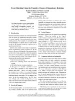
The Markov field depicted in Figure 1 is represented
by an undirected graph because conditional indepen-
dence is a symmetric relationship. But decomposable
models can also be characterized by directed graphs and
interpreted according to the semantics of a Bayesian
network ([21]; also described as "recursive causal mod-
els" in [27] and [16]). In a Bayesian network, the no-
tions of causation and influence replace the notion of
conditional independence in a Markov field. The par-
ents of a variable (or set of variables) V are those vari-
ables judged to be the direct causes or to have direct
influence on the value of V; V is called a "response"
to those causes or influences. The Bayesian network
representation of a decomposable model embodies an
explicit ordering of the n variables in the model such
that variable i may be considered a response to some
or all of variables {i + 1, , n}, but is not thought of
as a response to any one of the variables {1 , i - 1}.
In all models presented in this paper, the sense tag of
the ambiguous word causes or influences the values of
all other variables in the model. The Bayesian network
representation of Model 4 is presented in Figure 2. In
Model 4, the variables in and percent are treated as in-
fluencing the values of rate, short, and pursue in order
to achieve an ordering of variables as described above.
142
[~~ LIPOS, L2POS
Figure 2
Comparison to Previous Work
Many researchers have avoided characterizing the inter-

actions among multiple contextual features by consider-
ing only one feature in determining the sense of an am-
biguous word. Techniques for identifying the optimum
feature to use in disambiguating a word are presented
in [7], [30] and [5]. Other works consider multiple con-
textual features in performing disambiguation without
formally characterizing the relationships among the fea-
tures. The majority of these efforts ([13], [31]) weight
each feature in predicting the sense of an ambiguous
word in accordance with frequency information, with-
out considering the extent to which the features co-
occur with one another. Gale, Church and Yarowsky
([10]) and Yarowsky ([29]) formally characterize the in-
teractions that they consider in their model, but they
simply
assume
that their model fits the data.
Other researchers have proposed approaches to sys-
tematically combining information from multiple con-
textual features in determining the sense of an ambigu-
ous word. Schutze ([26]) derived contextual features
from a singular value decomposition of a matrix of letter
four-gram co-occurrence frequencies, thereby assuring
the independence of all features. Unfortunately, inter-
preting a contextual feature that is a weighted combina-
tion of letter four-grams is difficult. Further, the clus-
tering procedure used to assign word meaning based on
these features is such that the resulting sense clusters
do not have known statistical properties. This makes it
impossible to generalize the results to other data sets.

Black ([3]) used decision trees ([4]) to define the re-
lationships among a number of pre-specified contextual
features, which he called "contextual categories", and
the sense tags of an ambiguous word. The tree construc-
tion process used by Black partitions the data according
to the values of one contextual feature before consider-
ing the values of the next, thereby treating all features
incorporated in the tree as interdependent. The method
presented here for using information from multiple con-
textual features is more flexible and makes better use
of a small data set by eliminating the need to treat all
features as interdependent.
The work that bears the closest resemblance to the
work presented here is the maximum entropy approach
to developing language models ([24], [25], [19] and [20]).
Although this approach has not been applied to word-
sense disambiguation, there is a strong similarity be-
tween that method of model formulation and our own.
A maximum entropy model for multivariate data is the
likelihood function with the highest entropy that satis-
fies a pre-defined set of linear constraints on the under-
lying probability estimates. The constraints describe
interactions among variables by specifying the expected
frequency with which the values of the constrained vari-
ables co-occur. When the expected frequencies speci-
fied in the constraints are linear combinations of the
observed frequencies in the training data, the resulting
maximum entropy model is equivalent to a maximum
likelihood model, which is the type of model used here.
To date, in the area of natural language processing,

the principles underlying the formulation of maximum
entropy models have been used only to estimate the
parameters of a model. Although the method described
in this paper for finding a good approximation to the
joint distribution of a set of discrete variables makes
use of maximum likelihood models, the scope of the
technique we are describing extends beyond parameter
estimation to include selecting the form of the model
that approximates the joint distribution.
Several of the studies mentioned in this Section have
used
interest
as a test case, and all of them (with the ex-
ception of Schutze [26]) considered four possible mean-
ings for that word. In order to facilitate comparison
of our work with previous studies, we re-estimated the
parameters of our best model and tested it using data
containing only the four LDOCE senses corresponding
to those used by others (usages not tagged as being one
of these four senses were removed from both the test
and training data sets). The results of the modified ex-
periment along with a summary of the published results
of previous studies are presented in Table 3.
While it is true that all of the studies reported in
Table 3 used four senses of
interest,
it is not clear that
any of the other experimental parameters were held con-
stant in all studies. Therefore, this comparison is only
suggestive. In order to facilitate more meaningful com-

parisons in the future, we are donating the data used in
this experiment to the Consortium for Lexical Research
(ftp site: clr.nmsu.edu) where it will be available to all
interested parties.
Conclusions and Future Work
• In this paper, we presented a method for formulating
probabilistic models that use multiple contextual fea-
tures for word-sense disambiguation without requiring
untested assumptions regarding the form of the model.
In this approach, the joint distribution of all variables
is described by only the most systematic variable in-
teractions, thereby limiting the number of parameters
to be estimated, supporting computational efficiency,
and providing an understanding of the data. Further,
different types of variables, such as class-based and
collocation-specific ones, can be used in combination
143
with one another. We also presented the results of a
study testing this approach. The results suggest that
the models produced in this study perform as well as
or better than previous efforts on a difficult test case.
We are investigating several extensions to this work.
In order to reasonably consider doing large-scale word-
sense disambiguation, it is necessary to eliminate the
need for large amounts of manually sense-tagged data.
In the future, we hope to develop a parametric model
or models applicable to a wide range of content words
and to estimate the parameters of those models from
untagged data. To those ends, we are currently investi-
gating a means of obtaining maximum likelihood esti-

mates of the parameters of decomposable models from
untagged data. The procedure we are using is a vari-
ant of the EM algorithm that is specific to models of
the form produced in this study. Preliminary results
are mixed, with performance being reasonably good on
models with low-order marginals (e.g., 63% of the test
set was tagged correctly with Model 1 using parame-
ters estimated in this manner) but poorer on models
with higher-order marginals, such as Model 4. Work is
needed to identify and constrain the parameters that
cannot be estimated from the available data and to de-
termine the amount of data needed for this procedure.
We also hope to integrate probabilistic disambigua-
tion models, of the type described in this paper, with a
constraint-based knowledge base such as WordNet. In
the past, there have been two types of approaches to
word sense disambiguation: 1) a probabilistic approach
such as that described here which bases the choice of
sense tag on the observed joint distribution of the tags
and contextual features, and 2) a symbolic knowledge
based approach that postulates some kind of relational
or constraint structure among the words to be tagged.
We hope to combine these methodologies and thereby
derive the benefits of both. Our approach to combining
these two paradigms hinges on the network representa-
tions of our probabilistic models as described in Section
4 and will make use of the methods presented in [21].
Acknowledgements
The authors would like to thank Gerald Rogers for shar-
ing his expertise in statistics, Ted Dunning for advice

and support on software development, and the members
of the NLP group in the CRL for helpful discussions.
References
[1] Baglivo, J., Olivier, D., and Pagano, M. (1992).
Methods for Exact Goodness-of-Fit Tests. Jour-
nal of the American Statistical Association, Vol.
87, No. 418, June 1992.
[2] Bishop, Y. M.; Fienberg, S.; and Holland, P
(1975). Discrete Multivariate Analysis: Theory
and Practice. Cambridge: The MIT Press.
[3] Black, Ezra (1988). An Experiment in Compu-
tational Discrimination of English Word Senses.
IBM Journal of Research and Development, Vol.
32, No. 2, pp. 185-194.
[4] Breiman, L., Friedman, J., Olshen, R., and Stone,
C. (1984). Classification and Regression Trees.
Monterey, CA: Wadsworth & Brooks/Cole Ad-
vanced Books & Software.
[5] Brown, P., Della Pietra, S., Della Pietra, V.,
and Mercer, R. (1991). Word Sense Disambigua-
tion Using Statistical Methods. Proceedings of the
29th Annual Meeting of the Association for Com-
putational Linguistics (A CL-91), pp. 264-304.
[6] Cowie, J., Guthrie, J., and Guthrie, L. (1992).
Lexical Disambiguation and Simulating Anneal-
ing. Proceedings of the 15th International Con-
ference on Computational Linguistics (COLING-
92). pp 359-365.
[7] Dagan, I., Itai, A., and Schwall, U. (1991). Two
Languages Are More Informative Than One. Pro-

ceedings of the 29th Annual Meeting of the Asso-
ciation for Computational Linguistics (A CL-9I),
pp. 130-137.
[8] Darroch, J., Lauritzen, S., and Speed, T. (1980).
Markov Fields and Log-Linear Interaction Models
for Contingency Tables. The Annals of Statistics,
Vol. 8, No. 3, pp. 522-539.
[9] Dunning, Ted (1993). Accurate Methods for the
Statistics of Surprise and Coincidence. Computa-
tional Linguistics, Vol. 19, No. 1, pp.61-74.
[10] Gale, W., Church, K., and
Yarowsky, D. (1992a).
A Method for Disambiguating Word Senses in a
Large Corpus. A T84T Bell Laboratories Statistical
Research Report No. 104.
[11] Gale, W., Church, K. and Yarowsky, D. (1992b).
Estimating Upper and Lower Bounds on the
Performance of Word-Sense Disambiguation Pro-
grams. Proceedings of the 30th Annual Meeting of
the A CL, 1992.
[12] Havranek, Womas (1984). A Procedure for Model
Search in Multidimensional Contingency Tables.
Biometrics, 40, pp.95-100.
[13] Hearst, Marti (1991). Toward Noun Homonym
Disambiguation Using Local Context in Large
Text Corpora. Proceedings of the Seventh Annual
Conference of the UW Centre for the New OED
and Text Research Using Corpora, pp. 1-22.
[14] Jorgensen, Julia (1990). The Psychological Real-
ity of Word Senses. Journal of Psycholinguistic

Research, Vol 19, pp. 167-190.
[15] Kelly, E and P. Stone (1979). Computer Recog-
nition of English Word Senses, Vol. 3 of North
Holland Linguistics Series, Amsterdam: North-
Holland.
[16] Kiiveri, H., Speed, T., and Carlin, J. (1984). Re-
cursive Causal Models. Journal Austral. Math.
Soc. (Series A), 36, pp. 30-52.
144
[17] Kilgarriff, Adam (1993). Dictionary Word Sense
Distinctions: An Enquiry Into Their Nature.
Computers and the Humanities,
26, pp.365-387.
[18] Koehler, K. (1986). Goodness-of-Fit Tests for
Log-Linear Models in Sparse Contingency Tables.
Journal of the American Statistical Association,
Vol. 81, No. 394, June 1986.
[19] Lau, R., Rosenfeld, R., and Roukos, S. (1993a).
Trigger-Based Language Models: a Maximum
Entropy Approach.
Proceedings of ICASSP-93.
April 1993.
[20] Lau, R., Rosenfeld, R., and Roukos, S. (1993b).
Adaptive Language Modeling Using the Max-
imum Entropy Principle.
Proc. ARPA Human
Language Technology Workshop.
March 1993.
[21] Pearl, Judea (1988).
Probabilistic Reasoning In

Intelligent Systems: Networks of Plausible Infer-
ence.
San Marco, Ca.: Morgan Kaufmann.
[22] Pederson, S. and Johnson, M. (1990). Estimating
Model Discrepancy.
Technometrics,
Vol. 32, No.
3, pp. 305-314.
[23] Procter, Paul et al. (1978).
Longman Dictionary
of Contemporary English.
[24] Ratnaparkhi, h. and Roukos, S. (1994). h Maxi-
mum Entropy Model for Prepositional Phrase At-
tachment.
Proc. ARPA Human Language Tech-
nology Workshop.
March 1994.
[25] Rosenfeld, R. (1994). h Hybrid Approach to
Adaptive Statistical Language Modeling.
Proc.
ARPA Human Language Technology Workshop.
March 1994.
[26] Schutze, Hinrich (1992). Word Space. In S.J.
Hanson, J.D. Cowan, and C.L. Giles (Eds.),
Ad-
vances in Neural Information Processing Systems
5, San Mateo, Ca.: Morgan Kaufmann.
[27] Wermuth, N. and Lauritzen, S. (1983). Graphi-
cal and recursive models for contingency tables.
Biometrika,

Vol. 70, No. 3, pp. 537-52.
[28] Wilks, Y., Fass, D., Guo, C., McDonald, J.,
Plate, T., and Slator, B. (1990). Providing Ma-
chine Tractable Dictionary Tools.
Computers and
Translation 2.
Also to appear in
Theoretical
and Computational Issues in Lexicai Semantics
(TCILS).
Edited by James Pustejovsky. Cam-
bridge, MA.: MIT Press.
[29] Yarowsky, David (1992). Word-Sense Disam-
biguating Using Statistical Models of Roget's
Categories Trained on Large Corpora.
Proceed-
ings of the 15th International Conference on
Computational Linguistics (COLING-92).
[30] Yarowsky, David (1993). One Sense Per Colloca-
tion.
Proceedings of the Speech and Natural Lan-
guage ARPA Workshop,
March 1993, Princeton,
NJ.
[31] Zernik, Uri (1990). Tagging Word Senses In Cor-
pus: The Needle in the Haystack Revisited.
Tech-
nical Report 90CRD198,
GE Research and Devel-
opment Center.

145
LDOCE Sense Representation Representation Representation
in Total Sample in Training Sample in Test Sample
sense 1: 361
"readiness to give attention" (15%)
sense 2: 11
"quality of causing attention to be given" (<1%)
sense 3: 66
"activity, subject, etc., which one (3%)
gives time and attention to"
271 90
(15% / (15%)
9 2
(<1%) (<1%)
50 16
(3%) (3%)
sense 4:
"advantage, advancement, or favor"
sense 5:
'% share (in a company, business, etc.)"
sense 6:
"money paid for the use of money"
178 130 48
(8%) (7%). (8%)
500 378 122
(21%) (21%) (20%)
1253 931 322
(53%) (53%) (54%)
Table 1: Distribution of sense tags.
Model Percent

Correct
1 P(rlpos, ilpos, ending,tag)
= 73%
P(rlposltag ) × P(ilposltag )× P(endingltag ) × P(tag)
2 P(rlpos, r2pos, llpos, 12pos, ending, tag) =
76%
P(rlpos, r2posltag ) × P(llpos, 12posltag)× P(endingltag) × P(tag)
3 P(percent,pursue, short, in, rate,tag)
= 61%"
P(shortlpercent, in, tag)x P(rate[percent, in, tag)x
P(pursuelPercent , in, tag)× P(percent, inltag) × P( tag)
4 P(percent, pursue, short, in, rate, rlpos, r2pos, llpos, 12pos, ending, tag)
= 78%
P( short[percent, in, tag) × P(ratelpercent, in, tag) × P(pursuelpercent, in, tag)×
P(percent, inltag)× P(rlpos, r2posltag ) × P(ilpos, 12posltag)× P(endingltag) × P(tag)
Table 2: The form and performance on the test data of the model found for each set of variables. Each of the
variables
short, in, pursue, rate(s), percent
(i.e., the sign '%') is the presence or absence of that spelling form. Each
of the variables
rlpos, r2pos, ilpos,
and
12pos
is the POS tag of the word 1 or 2 positions to the left (/) or right (r).
The variable
ending
is whether
interest
is in the singular or plural, and the variable
fag

is the sense tag assigned to
interest.
Model Percent
Correct
Black (1988) 72%
Zernik (1990) 70%
Yarowsky (1992) 72%
Bruce & Wiebe
model 4 using only four senses 79%
Table 3: Comparison to previous results.
146