Comprehensive two-dimensional liquid chromatography of heavy oil

Journal of Chromatography A, 1564 (2018) 110–119

Contents lists available at ScienceDirect

Journal of Chromatography A
journal homepage: www.elsevier.com/locate/chroma

Comprehensive two-dimensional liquid chromatography of heavy oil
Fleur T. van Beek a,b,∗ , Rob Edam c , Bob W.J. Pirok a,b , Wim J.L. Genuit c ,
Peter J. Schoenmakers a
a
Universiteit van Amsterdam, Van’ t Hoff Institute for Molecular Sciences, Analytical-Chemistry Group, Science Park 904, 1098 XH, Amsterdam, The
Netherlands
b
TI-COAST, Science Park 904, 1098 XH Amsterdam, The Netherlands
c
Shell Global Solutions International B.V., Grasweg 31, 1031 HW, Amsterdam, The Netherlands

a r t i c l e

i n f o

Article history:
Received 22 February 2018
Received in revised form 1 June 2018
Accepted 3 June 2018
Available online 5 June 2018
Keywords:
Short residue
PAH
Vacuum distillation

De-asphalted heavy oil
PIOTR
SARA

a b s t r a c t
Heavy oil refers to the part of crude oil that is not amenable to further distillation. Processing of
these materials to useful products provides added value, but requires advanced technology as well as
extensive characterization in order to optimize the yield of the most profitable products. The use of
comprehensive two-dimensional liquid chromatography (LC × LC) was investigated for the characterization of de-asphalted short residue, also called maltenes. Initial studies were performed on a polycyclic
aromatic hydrocarbon standard, an aromatic extract of hydrowax, and the fractions obtained after solvent fractionation of the maltenes. Cyanopropyl- and octadecyl-silica were used as first-dimension and
second-dimension columns, respectively. The analysis of the maltenes and fractions thereof required
a change in first-dimension stationary phase to biphenyl as well as an increase in modifier strength
to improve recovery. The extensive characterization of maltenes with LC × LC within four hours was
demonstrated.
The Program for the Interpretive Optimization of Two-dimensional Resolution (PIOTR) has been applied
to aid the method development, but due to the absence of specific peaks in the chromatograms it was
challenging to apply to the maltenes or its fractions. Nonetheless, an approach is suggested for resolution
optimization in cases such as the present one, in which regions of co-elution are observed, rather than
clearly separated peaks.
© 2018 The Author(s). Published by Elsevier B.V. This is an open access article under the CC BY license
( />
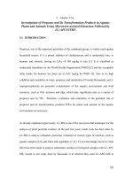
1. Introduction
A part of heavy oil is the short residue, also called vacuum
residue or vacuum bottoms. This is the solid hydrocarbon that
remains at the bottom of a vacuum distillation column after the
volatile material has removed at reduced pressure (Fig. 1). Extracting higher value products out of this material requires additional
processing using delayed coking technology, such as Exxon’s Flexicoker [1] or Shell’s Hycon [2]. To optimize the yield of the most
profitable products from these processes, the material needs to be
thoroughly characterized in order to optimize the conversion process [3]. The characterization of the short residue still has room for
improvement, although optimization is definitely a challenge.

Since the molecular composition of short residue is so complex,
the material is often separated before analysis into sub-fractions

∗ Corresponding author at: Science Park 904, Amsterdam, 1098 XH, The
Netherlands.
E-mail address: (F.T. van Beek).

based on solubility behavior [4,5]. One of the main methods for this
is a liquid chromatographic (LC) method known as SARA analysis, in
which a hydrocarbon mixture is separated into four fractions: Saturates, Aromatics, Resins, and Asphaltenes [6]. The saturate fraction
includes alkanes (paraffins) and cyclic alkanes (naphthenes). The
aromatic fraction consists of molecules incorporating at least one
aromatic ring. The resin fraction consists of compounds that contain heteroatoms, hence it is often referred to as the polar fraction
or the “polars”. This is evident by the fractionation process as the
resins stick to the stationary phase until (back)flushing with a relatively polar solvent, such as dichloromethane (DCM). Asphaltenes
are defined by their solubility range. They are soluble in toluene, but
precipitate upon addition of excess n-heptane or n-pentane [7]. One
has to be aware that SARA fractions are never completely excised
from one another [8]. This remains inevitable when employing
solvent fractionation. Understanding the composition of a specific
SARA fraction can provide valuable insights, whilst retaining much
of the sample dimensionality [9], and provide feedback for further
processing of the short residues into profitable products.

/>0021-9673/© 2018 The Author(s). Published by Elsevier B.V. This is an open access article under the CC BY license ( />

F.T. van Beek et al. / J. Chromatogr. A 1564 (2018) 110–119

Fig. 1. Schematic of a petroleum refinery, adapted from Speight et al. [6].

For the analysis of heavy oils many techniques have been
applied, including Fourier-transform ion-cyclotron-resonance
mass spectrometry (FT-ICR MS) [10–12], high-temperature comprehensive two-dimensional gas chromatography (HT-GC × GC)
[13,14] and comprehensive two-dimensional supercritical-fluid
chromatography (SFC × SFC) [15,16]. Dutriez et al. [17] analyzed
resin fractions using both FT-ICR MS and HT-GC × GC in order to
compare the analytical capabilities of these techniques for heavy
oils. However, as the components become heavier and less volatile,
their analysis becomes more difficult. Volatility of a sample is
an inherent requirement for gas chromatography (GC) and since
this property decreases as the molar masses and polarity of oil
components increases, GC × GC becomes more complicated and
eventually impossible for materials such as short residue. FT-ICR
MS is able to deal better with heavier samples, but struggles with
accurate quantification and with the separation of isomeric components. Techniques like supercritical-fluid chromatography (SFC)
and LC are better suited for characterizing short residue, since they
do not require volatile analytes. Nevertheless, the analysis of heavy
components heavier than C90 is troublesome for SFC [16].
While one-dimensional liquid chromatography (1D-LC) is most
often employed for sample preparation and fractionation of heavy
hydrocarbons, comprehensive component analysis is impossible
due to broad, unresolved peaks in the chromatogram caused by
the molecular complexity of the sample [18,19]. The purpose of
this work is to determine if comprehensive two-dimensional liquid
chromatography (LC × LC) could be a possible alternative approach.
LC × LC is a method in which the first-dimension (1 D) chromatographic column is coupled to a second-dimension (2 D)
chromatographic column through a switching valve or another
transferring device in order to subject the entire 1 D effluent to 2 D
separations [20,21]. The effluent from the 1 D should be sampled 2–4
times over the 4-␴ width of the 1 D peak to ensure two-dimensional

resolution [22,23]. In LC × LC the peak capacities of the two dimensions can ideally be multiplied, giving rise to an immense increase
in separation power [18,23,24]. In order to deal with complex samples that require more peak capacity than an LC method can offer,
LC × LC seems to provide good prospects. Duarte et al. [25] applied
LC × LC on natural organic matter, where 1D-LC could not handle
the sample complexity, and showed great improvement in their
ability to resolve individual components in the sample. Similarly,
Murahashi [26] performed LC × LC on polycyclic aromatic hydrocarbons (PAHs) in environmental samples and showed that the
technique provided valuable additional information. More specifically, Jakobsen et al. [27] applied LC × LC with pulsed elution of the
first dimension to a heavy oil fraction of vacuum gas oil and coker
gas oil.
Nevertheless, the advantages of the additional dimension in
LC × LC come at the cost of significantly more complicated method
development [21,28–30]. As the two columns are coupled through
a modulation device, often consisting of a switching valve and two
loops that are filled and emptied consecutively, the optimization
of both separations is no longer independent. Similar to 1D-LC,
LC × LC also requires optimization of individual parameters, such
as column dimensions, particle size, flow rate, mobile-phase com-

111

position, temperature, pH, etc. In addition, LC × LC requires the
compatibility of the two dimensions and the way they are connected to be considered, i.e. modulation time and the effects of the
1 D effluent on the 2 D separation [31]. Recently described software
called “Program for Interpretive Optimization of Two-dimensional
Resolution” (PIOTR) developed by Pirok et al. [32] was shown to
speed up LC × LC method development, based on only a few experiments, taking into account the retention behavior of the analytes
under varying isocratic or gradient mobile-phase conditions.
Vanhoenacker et al. [33] achieved a separation of a petroleum
short residue by multiple-heart-cut two-dimensional liquid chromatography (2D-LC), using a combination of normal-phase LC

(NPLC) and reversed-phase LC (RPLC). Although they were specifically interested in the quantification of PAHs to deal with
regulations, their work suggested that comprehensive twodimensional separation of short residues could provide a more
complete overview of sample composition. In fact, Vanhoenacker
et al. [34] investigated LC × LC of the aromatic fraction of mineral
oil after liquid-liquid extraction using n-hexane and nitromethane.
Although this method provided more comprehensive information
on the sample, the mineral-oil fraction studied was probably still
light enough to enable analysis by the previously mentioned methods, i.e. FT-ICR/MS and HT-GC × GC, which are more mature and
already used routinely. To the authors’ knowledge the application
of LC × LC to short residue fractions has not been reported previously.
In this work, an LC × LC method has been developed to separate the saturate, aromatic and resin fractions of de-asphalted short
residue in order to provide feedback for oil processing. To streamline method development and to test the efficacy of the available
software, PIOTR [32] was applied in the current work.
2. Material and methods
2.1. Instrumental
The main instrument used in this study was an Agilent
1290 Infinity II 2D-LC Solution (Agilent, Germany). The system
included two binary pumps (G7120 A) with V35 Jet Weaver mixers
(G4220-60006), a multisampler (G71678), two thermostatted column compartments (G71168) equipped with a 2-pos/6-port valve
(5067-4137) and 2-pos/8-port valve (5067-4214) fitted with two
40-␮L loops, and a diode-array detector (DAD; G7117B) fitted with
a Max-Light Cell (G4212-60008). After the DAD a Thermo Scientific Dionex Corona Veo RS charged-aerosol detector (CAD) was
attached, through a T-piece with a pressure release (G4212-68001),
which communicated with the system through a transformer box
(G13908).
An Agilent stable-bond cyanopropyl column (CN; 100 × 2.1 mm,
3.5 ␮m), or a Phenomenex Kinetex pentafluorophenyl column (F5;
100 × 3.0 mm, 2.6 ␮m), or a Phenomenex Kinetex biphenyl column (BiPh; 100 × 3.0 mm, 2.6 ␮m) was used in the first dimension.
An Agilent Zorbax RRHD Eclipse PAH column (C18 ; 50 × 3.0 mm,
1.8 ␮m) was used in the second dimension.

The system was controlled by Agilent OpenLAB CDS Chemstation Edition A02.02 software. Data were collected using Agilent
OpenLAB CDS ChemStation Edition for LC & LC/MS Systems, Version C.01.07 [27] with Agilent 1290 Infinity 2D-LC Software, Version
A.01.02[025]. Data was processed using MatLAB R2015a version
8.5.0.197613 (Mathworks, Woodshole, MA, USA).
2.2. Chemicals
2-Propanol (IPA, gradient grade), acetonitrile (ACN, Reag. Ph Eur
gradient grade), dichloromethane (DCM, for liquid chromatogra-


112

F.T. van Beek et al. / J. Chromatogr. A 1564 (2018) 110–119

phy), methanol (MeOH, Reag. Ph Eur gradient grade), and toluene
(for liquid chromatography) were LiChrosolv purchased from
Merck (Darmstadt, Germany). Deionized water was prepared using
a MilliQ Integral A-10 system from Merck.
2.3. Samples
The oil samples were obtained from Shell Global Solutions International B.V. in Amsterdam, The Netherlands. After asphaltene
removal according to ASTM method D3279 [7], the remaining deasphalted short residue, referred to as maltenes, was fractionated
according to an in-house SARA fractionation method to obtain the
saturate, aromatic and resin fractions. The samples were dissolved
in toluene to a concentration of 20 mg/mL. The aromatic extract
of hydrowax (HW) was obtained by liquid-liquid extraction with
DMSO. A 24-component polycyclic aromatic hydrocarbon standard
mix, as tested in EPA method 610 (PAH610), was obtained from
Accustandard (p.n. M-8100-QC, New Haven, Connecticut, USA).
This PAH610 standard contained polycyclic aromatic hydrocarbons
ranging from 2-ringed structures up to 6-ringed structures, including a few nitrated and methylated compounds.
2.4. Methods

2.4.1. 1D-LC methods
For comparison of the 1 D stationary phases the column ovens
were set to 40 ◦ C and the acquisition rate of the DAD was set to
80 Hz, with a 4 nm slit width to collect data at wavelengths of 220,
254, 280, 305, 340, and 500 nm. The injection volume was 0.1 ␮L.
Different mobile-phase compositions were used; water (A) and
ACN (B), water (A) and MeOH (B), or water/MeOH 50:50 (v/v) (A)
and THF (B) for the respective investigations into modifier influence.
The BiPh and F5 columns were used at a flow rate of 0.6 mL/min.
For the modifiers ACN and MeOH the gradient programs were:
0–0.05 min, isocratic at 50%B; 0.05–32.05 min, linear gradient to
100%B; 32.05–55 min, isocratic at 100%B; 55–56 min, linear gradient to 50%B; 56–60 min, isocratic at 50%B. For the THF modifier, the
gradient program was somewhat different to reflect the greater
eluent strength of solvent A: 0–0.05 min, isocratic at 100%A;
0.05–32.05 min, linear gradient to 100%B; 32.05–55 min, isocratic
at 100%B; 55–56 min, linear gradient to 100%A; 56–60 min, isocratic
at 100%A.
Due to a lower maximum pressure tolerance of the CN column
compared to the BiPh and F5 columns a flow rate of 0.4 mL/min
was used when testing the CN column. In order to keep the
number of column volumes consistent with those of the other
columns, the gradient programs for the modifiers ACN and MeOH
were: 0–0.04 min, isocratic at 50%B; 0.04–23.6 min, linear gradient to 100%B; 23.6–40.4 min, isocratic at 100%B; 40.4–41.1 min,
linear gradient to 50%B; 41.1–44.1 min, isocratic at 50%B. Again
accounting for the greater eluent strength, the gradient program for the THF modifier was: 0–0.04 min, isocratic at 100%A;
0.04–23.6 min, linear gradient to 100%B; 23.6–40.4 min, isocratic
at 100%B; 40.4–41.1 min, linear gradient to 100%A; 41.1–44.1 min,
isocratic at 100%A.
The 1D-LC separation of HW was performed at 40 ◦ C with a flow
rate of 0.85 mL/min on the C18 column (see Section 2.1). The acquisition rate of the DAD was set to 80 Hz with a 4 nm slit width to

collect at wavelengths of 220 nm and 340 nm. The injection volume was 0.1 ␮L. The mobile phase consisted of water (A) and ACN
(B), which were combined in a gradient program: 0-0.05 min, isocratic at 40%B; 0.05–12 min, linear gradient to 100%B; 12–18 min,
isocratic at 100%B; 18–20 min, linear gradient to 40%B; 20–24 min,
isocratic at 40%B.

2.4.2. LC × LC of aromatic extract of hydrowax and aromatic
fraction of maltenes
The initial LC × LC method, applied to the HW sample and the
aromatic fraction of maltenes, employed a CN and a C18 stationary phase in the 1 D and 2 D, respectively. The dwell volumes for
the 1 D and 2 D were 174 ␮L and 190 ␮L respectively. UV data were
recorded at 220, 254, 280, 305, 340 nm at 80 Hz and CAD data was
recorded at 100 Hz in the 0–500 pA range. The injection volume
was set to 1.0 ␮L. The temperature of both thermostatted column
compartments was set to 40 ◦ C. The 1 D mobile phase was water (A)
and ACN (B). The flow rate was set to 20 ␮L/min with the following
a gradient program: 0–2 min, isocratic at 50%B; 2–242 min, linear
gradient to 100%B; 242–332 min, isocratic at 100%B; 332–338 min,
linear gradient to 50%B; 338–355 min, isocratic at 50%B. The 2 D
mobile phase was MeOH (A) and DCM (B). The flow rate was set to
2.0 mL/min with the following gradient program: 0–1.3 min, linear
gradient from 0% to 65%B; 1.3–1.35 min, linear gradient to 100%A;
1.35–1.5 min, isocratic at 100%A. This gradient was repeated from
0 to 337.5 min of the analysis with a modulation time of 1.5 min.

2.4.3. LC × LC for PIOTR
For both the HW and PAH610, the same methods were used
to generate peak data as input for PIOTR. Both methods were performed at 40 ◦ C employing a CN and a C18 stationary phase as 1 D
and 2 D, respectively. The injection volume of HW and PAH610 were
1.0 ␮L and 0.5 ␮L respectively. UV data was recorded at 220, 254,
280, 305, 340, and 500 nm at 80 Hz and CAD data was recorded

at 25 Hz in a 0–500 pA range. The 1 D used water (A) and ACN (B)
at a flow rate of 10 ␮L/min, whilst the 2 D used MeOH (A) and
DCM/MeOH 90:10 (v/v) (B) at a flow rate of 2.0 mL/min.
For the ‘fast’ PIOTR method employing a steep gradient, the
1 D gradient was programmed to 180 min: 0–2 min, isocratic at
50%B; 2–150 min, linear gradient to 100%B; 150–167 min, isocratic
at 100%B; 167–175 min, linear gradient to 50%B; 175–180 min,
isocratic at 50%B. The 2 D was programmed to modulate up to
180 min with a modulation time of 1 min: 0-0.9 min, linear gradient from 100%A to 100%B; 0.9-0.95 min, linear gradient to 100%A;
0.95–1 min, isocratic at 100%A.
For the ‘slow’ PIOTR method employing a shallower gradient,
the 1 D gradient was programmed to 540 min: 0–2 min, isocratic at
50%B; 2–450 min, linear gradient to 100%B; 450–500 min, isocratic
at 100%B; 500–525 min, linear gradient to 50%B; 525–540 min,
isocratic at 50%B. The 2 D was programmed to modulate up to
540 min with a modulation time of 3 min: 0–2.7 min, linear gradient from 100%A to 100%B; 2.7–2.85 min, linear gradient to 100%A;
2.85–3 min, isocratic at 100%A.

2.4.4. Optimum LC × LC method for aromatic extract of hydrowax
The optimum method determined by PIOTR, applied to HW
was performed using the same columns, mobile phases, injection volume, and data acquisition conditions as those applied
in the PIOTR experiments (see Section 2.4.3). The 1 D flow rate
was set to 15 ␮L/min with the following a gradient program:
0–1 min, isocratic at 50%B; 1–101 min, linear gradient to 100%B;
101–158 min, isocratic at 100%B; 158–159 min, linear gradient to
50%B; 159–160 min, isocratic at 50%B. The 2 D flow rate remained
the same at 2.0 mL/min but now followed the gradient program: 00.2 min, isocratic at 100%A; 0.2–1.2 min, linear gradient to 11%B;
1.2–1.4 min, linear gradient to 100%B; 1.4–1.92 min, isocratic at
100%B; 1.92–1.95 min, linear gradient to 100%A; 1.95–2 min, isocratic at 100%A. This gradient was repeated from 0 to 160 min of
the analysis with a modulation time of 2 min.

F.T. van Beek et al. / J. Chromatogr. A 1564 (2018) 110–119

2.4.5. Optimum LC × LC method for polycyclic aromatic
hydrocarbon standard PAH610
The optimum method determined by PIOTR, applied to PAH610
was also performed using the same columns, mobile phases, and
data acquisition conditions as those applied in the PIOTR experiments (see Section 2.4.3). The injection volume was 1.0 ␮L. The
1 D flow rate was set to 20 ␮L/min with the following a gradient
program: 0–10 min, isocratic at 50%B; 10–70 min, linear gradient
to 70%B; 70–118 min, isocratic at 70%B; 118–119 min, linear gradient to 50%B; 119–120 min, isocratic at 50%B. The 2 D flow rate
again remained the same at 2.0 mL/min, but flowed the gradient
program: 0-0.1 min, isocratic at 100%A; 0.1-0.95 min, linear gradient to 2.3%B; 0.95–1 min, linear gradient to 100%A. This gradient
was repeated from 0 to 120 min of the analysis with a modulation
time of 1 min.

2.4.6. LC × LC method for maltenes and its SARA fractions
The final LC × LC method, applied to the maltenes and its SARA
fractions employed a BiPh and C18 stationary phase as 1 D and
2 D, respectively. The flow rates, column temperature, and data
acquisition conditions were the same as those used initially (see
Section 2.4.2), but the injection volume was increased to 10 ␮L.
The 1 D mobile phase was MeOH (B) and THF (A) and followed the
gradient program: 0–260 min, linear gradient from 0% to 100%A;
260–270 min, isocratic at 100%A; 270–275 min, linear gradient
to 100%B; 275–280 min isocratic at 100%B. The 2 D mobile phase
remained the same using of MeOH (A) and DCM/MeOH 90:10 (v/v)
(B). The gradient was programmed to modulate up to 276 min with
a modulation time of 1.5 min: 0–1.3 min, linear gradient from 0% to

100%B; 1.3–1.35 min, isocratic at 100%B; 1.35–1.5 min linear gradient to 0%B.

3. Results and discussion
In industry, structure-property relationships based on compositional information, beyond straightforward solvent fractionation,
are crucial to successfully process short residue into useful products. In the case of short residue it is difficult to obtain meaningful
information from a 1D-LC experiment. A typical 1D-LC method for
heavy aromatics has been described by Fetzer et al. [35], where
the large PAHs were monitored at 305 and 340 nm. Since key
components to be measured co-elute with other components in
1D-LC, jeopardizing the accuracy of the analysis, LC × LC analysis
was attempted in this work to improve the separation. Although
the 1D-LC separation in Fig. 2A is clearly superior to the reconstituted 1D-LC of the same column in LC × LC (shown to the left of the
LC × LC chromatogram in Fig. 2B), one must take into account the
compromises that need to be made in order to make the LC × LC
separation possible and competitive to 1D-LC. Theoretical calculation of the peak capacity in 1D-LC gives an approximate value of 50,
whereas the peak capacity in LC × LC is the product of both dimensions giving an approximate peak capacity of 875. Even though
the separation space is not entirely utilized, the possible gain in
separation is still major. As seen in Fig. 2A, 1D-LC of HW shows a
great deal of overlap between peaks and poor or no baseline resolution. The heavier components of interest, eluting after 10 min,
overlap with other components and show poor baseline resolution,
which makes quantification difficult. These components are clearly
separated using LC × LC as seen in Fig. 2B, where the heavier components elute as peaks fully resolved from the bulk. Therefore, a
two-dimensional approach may result in more-accurate identification and quantitation of the high-molecular-mass aromatics.

113

3.1. Optimization of separations of PAH610 and HW using PIOTR
Although applying an LC × LC method to HW showed that this
can provide added value, optimizing such a method takes a long
time. This is not favourable in industry. A sub-optimal, robust and

reliable method may often be accepted, avoiding the costs associated with optimizing a method during several months. This is one of
the reasons for which the “Program for Interpretive Optimization
of Two-dimensional Resolution” (PIOTR) was developed by Pirok
et al. [32]. The program requires retention data of a number of
compounds of interest obtained from two LC × LC chromatograms
with sufficiently different gradient slopes in each dimension to
establish retention-model parameters. These parameters can be
used to predict the retention times under any type of mobilephase-composition program. The various method parameters are
optimized by simulating a large number of methods, after which
the analyst may assess the separation performance by evaluation
of quality descriptors (e.g. orthogonality, resolution and analysis
time) through Pareto-optimality (PO) plots. PO plots can be used to
display only the Pareto front, i.e. those points for which the different
criteria cannot all be improved simultaneously. For example, in a PO
plot with analysis time and resolution as criteria, only those points
are retained at which better resolution in a shorter time cannot be
achieved.
It was decided to test the program on a standard PAH sample (PAH610), as well as on the HW sample. Fig. 3 shows the
fast and slow chromatograms obtained for the optimization by
PIOTR and the chromatogram collected after applying the optimized method to PAH610 (3 A, 3B and 3C respectively) and HW (3D,
3E, and 3 F respectively). Both of the optimized methods require a
shorter analysis time. The optimized method for PAH610 clearly
shows increased resolution and orthogonality, whereas the optimized method for HW mainly led to improvements in terms of
analysis time and orthogonality.
Using the data from Figs. 3A, B, D and E, PO-plots were automatically generated by PIOTR for all possible combinations of
input parameters, as can be seen in Fig. 4A, in which the possible
outcomes for the optimization of PAH610 are depicted. The paretooptimal front is highlighted by a red dashed line and the selected
optimum method was a point on the Pareto-optimal front indicated
by a yellow circle and pointed out by the arrow. This method was
only one out of a range of possible methods and was selected based

on a combination of resolution, orthogonality and analysis time.
The optimization approach focused on the parameters of orthogonality, resolution and analysis time. The measure of resolution was
calculated as described by Pirok et al. [32], in short the resolution
of a peak is calculated in relation to all other peaks in the chromatogram. Since PIOTR allows the user to inspect every PO point
and make a decision based on the scores and attractiveness of the
chromatogram, a balance could be found between analysis time,
resolution and orthogonality. The decision of selecting a point in
the PO-plot remains that of the analyst and could be revisited if the
validation fails or if the analytical question changes.
The experimentally obtained “optimal” method was compared
with the theoretical prediction using the experiment-verification
tool, which allows one to determine whether the predicted and
experimental results concur or deviate significantly. Deviations
between the predicted and experimental results may indicate
misassignments during peak tracking, imperfect retention models or experimental variability. Fig. 4B shows the validation plot
of PAH610 given by PIOTR in which the experimentally obtained
peaks have been selected as points. The black circles connected to
the experimental points depict the retention times of the corresponding peaks as predicted by PIOTR. The plot is supported by a
validation table, seen in the supplementary information S3, which
indicates the difference between the experimental and predicted


114

F.T. van Beek et al. / J. Chromatogr. A 1564 (2018) 110–119

Fig. 2. (A) LC-UV chromatogram of HW shown at a detection wavelength of 340 nm, recorded according to the method described in Section 2.4.1 using the same C18 column
as in the second dimension of the LC × LC analysis. (B) LC × LC-UV chromatogram of HW, shown at a detection wavelength of 340 nm, recorded according to the method
described in Section 2.4.2. The LC-UV chromatograms to the left and top of the LC × LC chromatogram have been reconstructed from the LC × LC data. Reconstruction was
performed by summing all intensities of the 1 D to obtain the (red) chromatogram to the left and summing all intensities of the 2 D to obtain the (green) chromatogram to the

top. For the full chromatograms see supplementary information S1.

Fig. 3. LC × LC-UV chromatograms of the fast (A), slow (B), and optimized (C) separations of PAH610 and the fast (D), slow (E), and optimized (F) separations of HW, shown
at a detection wavelength of 340 nm. The chromatograms were recorded according to the methods described in Sections 2.4.3, 2.4.4, and 2.4.5. For the full chromatograms
see supplementary information S2.

data numerically. The differences in the current example seem to be
small, except around 50 min in 1 D, where the experimental peaks
and predicted points (depicted as black circles) are quite far apart
as indicated by the long (red) lines. This may be due to the fact that
the gradient parameters of the predicted optimal method were not
within the domain of the scanning gradients used to determine the
retention parameters, which has very recently been shown to affect
the accuracy of prediction [36].

3.2. LC × LC of SARA fractions
LC × LC provides added value to the separation of HW, since
many components co-eluting in 1D-LC can now be separated. When
LC × LC is applied to heavier, more complex samples, such as SARA
fractions the outcome may be less clear. The boiling-point range
of a short residue starts at 470 ◦ C under vacuum conditions. In
this domain the numbers of isomers present ranges in the billions


F.T. van Beek et al. / J. Chromatogr. A 1564 (2018) 110–119

115

Fig. 4. (A) Pareto optimality plot for PAH610 showing the pareto-optimal front (red dashed line) and the point selected as the optimum method (yellow circle indicated with
arrow). (B) LC × LC-UV chromatogram of the optimized separation of PAH610 shown at a detection wavelength of 340 nm. The black dots indicate the points at which the

corresponding peaks eluted according to the prediction by PIOTR. See supplementary information S3 for the complete table of data points.

[37]. By taking the aromatic SARA fraction of a de-asphalted short
residue as an intermediate sample, the number of components is
reduced. However, the sample complexity remains high. Beside the
many aromatic components, some saturate and resin components
may still be present due to the nature of the solvent-fractionation
process.
As can be seen from Fig. 5, a method similar to that applied to
HW does not result in the elution of the entire aromatic SARA fraction. Nevertheless, some potentially useful separation is observed,
which may reveal underlying information about the composition of
this particular fraction. One can observe at least three main regions
that have been separated; a fanned out pattern similar to HW indicated by the red dotted line; a broad stretched out diagonal smear;
and a thin tail indicated by the pink dashed line. Further study of
the fractions eluting in the different regions using MS may provide more insight in the separation, but this was not the aim of the
present study. Although the identification of components in this
separation was not performed, the comparison of samples from different origins may give a quick indication of the variations between
them.

supplementary information S4. Fig. 7 shows a comparison of the
chromatograms obtained with gradients from water/MeOH 50:50
(v/v) to MeOH (red, dashed line), water/ACN 50:50 (v/v) to ACN
(blue, dotted line) and MeOH to THF (green, solid line) to elute the
aromatic fraction of maltenes. Although the elution window is narrowed using THF, a much greater fraction of the sample is seen to
elute. The signal returns to the baseline early, suggesting complete
elution of the sample. The disturbance in the signal between 1 and
5 min is due to the oversaturation of the detector from the sample
solvent toluene, which is evident after subtraction of the blank. The
modifier comparison is similar for the CN and F5 stationary phases,
which can be seen in supplementary information S5.

Although the optimization of the first dimension was crucial to
allow all of the sample to elute, the second-dimension performance
was found to be adequate for application. A polymeric C18 stationary phase was used because of its additional shape selectivity and
better resolution in comparison with typical C18 stationary phases,
as explained by Sander and Wise [38,39].

3.3. Stationary- and mobile-phase optimization for LC × LC of
maltenes

The new LC × LC method for separating the SARA fractions
appeared to elute all of the components and the results, seen in
Fig. 8, suggested that the fractions could be separated from each
other. In order to detect the saturated components a chargedaerosol detector (CAD) was added after the UV detector. This led
to the interesting observation of a bimodal distribution for the
saturate fraction, which suggests significant differences between
the various saturated components. Although the separation of the
fractions may not seem all that great, one must realize that the
number of components present is extremely high [37]. The required
peak capacity to resolve all these compounds is currently impossible to reach, leading to smeared out regions rather than sharp
peaks. Interestingly, the slope of the aromatics band (Figs. 8B and E)
seems somewhat steeper than that of the other fractions, suggesting a higher retention of aromatic compounds on the C18 stationary
phase.
To indicate whether it would be possible to separate the fractions of maltenes within one run, the separations were overlaid
using the contours of the fractions in the CAD data, see Fig. 9A.
Additionally, the maltenes sample from which the fractions were
separated was injected in the LC × LC system and detected using
UV, see Fig. 9B, and CAD, see Fig. 9C. From these results is can be
seen that there is good separation of the saturate fraction, but that
the aromatic and resin fraction still appear to co-elute. This may be

Our aim was to analyse a maltenes sample in one run using
LC × LC. Such a de-asphalted short residue contains a myriad of
compounds, including apolar and polar components. These are
expected to elute both before and after the components eluting
from the aromatic fraction of maltenes seen in Fig. 5. To develop
a method tailored to the maltenes sample, an initial optimization
of stationary and mobile phases was performed. The optimization
focussed on the first dimension, which was deemed to be the limiting factor with respect to the recovery of the sample. We aimed to
maximize the orthogonality of the two separations, without turning to NPLC, as this would not be compatible with the RPLC second
dimension. A few alternative stationary phases were compared
using different modifiers. Fig. 6 shows the separation of PAH610
on a CN (red, dashed line), an F5 (green, dotted line), and a BiPh
(blue, solid line) stationary phase using identical mobile-phase conditions.
To enhance the recovery, purging with a strong solvent is
required. In the present case THF was investigated for this purpose.
The F5 and BiPh stationary phases showed sufficient retention.
The latter stationary phase was selected, since it possessed the
highest column efficiency. For the performance-test results see

3.4. LC × LC of maltenes


116

F.T. van Beek et al. / J. Chromatogr. A 1564 (2018) 110–119

Fig. 5. LC × LC-UV chromatogram of an aromatic fraction of maltenes, recorded at a detection wavelength of 254 nm. Besides the main smear two different regions have been
indicated by the red dotted line and the pink dashed line. The chromatogram was recorded according to the method described in Section 2.4.2.

Fig. 6. LC-UV chromatograms of PAH610 separated on a CN (red, dashed line), an F5 (green, dotted line) and a BiPh (blue, solid line) stationary phase, shown at a detection

wavelength of 254 nm. The separations were performed according to the methods described in Section 2.4.1. The retention axes were normalized by conversion to number of
column volumes. The signal intensity of the F5 (green, dotted line) and CN (red, dashed line) measurements were increased by 1500 and 3000 mAU respectively for plotting.

Fig. 7. LC-UV chromatograms of an aromatic fraction of maltenes, shown at a detection wavelength of 254 nm, using 60 min linear gradients from water/MeOH 50:50 (v/v)
to MeOH (red, dashed line), water/ACN 50:50 (v/v) to ACN (blue, dotted line) and MeOH to THF (green, solid line). The separations were performed according to the methods
described in Section 2.4.1.

explained by the sheer number of compounds present. Nevertheless, the separation power of this system, using the current column
combination and conditions, seems insufficient to fully differentiate between the aromatic and resin fractions.

Optimizing the gradients of this LC × LC method could improve
the separation and may slightly pull apart the different groups.
However, PIOTR has never been applied to this type of sample, since it requires individual peaks to be tracked to determine


F.T. van Beek et al. / J. Chromatogr. A 1564 (2018) 110–119

117

Fig. 8. LC × LC-UV chromatograms of the saturate (A), aromatic (B) and resin (C) fractions of maltenes, shown at a detection wavelength of 340 nm, and LC × LC-CAD
chromatograms of the saturate (D), aromatic (E) and resin (F) fractions of maltenes. The chromatograms were recorded according to the method described in Section 2.4.6.

Fig. 9. (A) Overlay of the contours of the saturate (green, solid line), aromatic (blue, dashed line) and resin (red, dotted line) fractions of maltenes detected using a CAD as seen
in Fig. 7. LC × LC-UV (B) chromatogram of the maltenes, shown at a detection wavelength of 340 nm and LC × LC-CAD (C) chromatogram of the maltenes. The chromatograms
were recorded according to the method described in Section 2.4.6.


118

F.T. van Beek et al. / J. Chromatogr. A 1564 (2018) 110–119

their retention parameters. Pinpointing the retention times of specific components in a sample which contains such a multitude of
components has been attempted by fractionating the sample and
re-injecting well-separated fractions into the fast and slow gradient runs, essentially creating artificial peak maxima. Since the peak
maxima of fractions will be selected as input rather than the peak
maxima of specific components, further investigation outside the
scope of this study is required to determine whether this approach
is applicable.

4. Conclusions
An initial separation of heavy oil using LC × LC has been
achieved. Saturates were separated from the aromatics and resins,
although, the latter were not resolved fully. The choice of stationary phases and the respective selectivity obtained for the samples
remain the limiting factors for obtaining informative separations.
PIOTR was applied to a standard mixture of polycyclic aromatic
hydrocarbons and to an aromatic extract of hydrowax. This showed
promise, but it is not yet possible to apply PIOTR to samples that
do not yield distinct peaks. To develop our understanding of the
maltenes further it would be useful to apply PIOTR. The retention
parameters obtained through this program can provide insight into
the behavior and, consequently, the nature of components within
a certain separation space. A possible way to enable the tracking of peaks between the fast and slow runs needed as input for
PIOTR would be to fractionate the sample. Re-injecting fractions
that were collected with sufficient time between them in both the
fast and slow run will allow tracking of the fraction maxima. PIOTR
could be applied on these maxima and be used to optimize the
gradients. Although this may seem like a simple solution it does
require quite a bit more time than just the collection of two LC × LC
chromatograms, which is one of the key assets of PIOTR.
Another way to improve our understanding of the maltenes

sample as well as its separation, would be to attach an MS to the
end of the system. However, the nature of the sample may complicate this hyphenation. The complexity of the sample and the
myriad of components present may cause matrix effects as well
as preferred or suppressed ionization of specific species. Nevertheless, the addition of the MS data would make the application of
PIOTR a lot easier, since it would allow for specific components to
be tracked according to their mass-to-charge ratio.

Acknowledgements
The authors wish to thank Gwen Philibert, Bob Szentirmay, Bill
Reppart and Ron Skelton from Shell Global Solutions International
(Houston, TX, USA) as well as the Amsterdam analytical team for
their interest and constructive feedback. Additionally the authors
would like to thank Frans van den Berg (formerly from Shell Global
Solutions International (Amsterdam, NL)) for making this research
possible.
This publication has been written within the context of the
MAnIAC project which is funded by the Netherlands Organization
for Scientific Research (NWO) in the framework of the Programmatic Technology Area PTA-COAST3 of the Fund New Chemical
Innovations [Project 053.21.113].

Appendix A. Supplementary data
Supplementary material related to this article can be found, in
the online version, at doi: />06.001.

References
[1] W.R. Epperly, L.E. Swabb, J.W. Taunton, Exxon donor solvent coal liquefaction
process, JPL Proc. Conf. Coal Use Calif. (1978) 268–272.
[2] B. Scheffer, M.A. Van Koten, K.W. Röbschläger, F.C. De Boks, The shell residue
hydroconversion process: development and achievements, Catal. Today 43
(1998) 217–224.

[3] J. Stommel, B. Snell, Consider better practices for refining operations,
Hydrocarb. Process. 86 (2007) 105–109.
[4] J.F. McKay, P.J. Amend, P.M. Harnsberger, T.E. Cogswell, D.R. Latham,
Separation and analyses of petroleum residues, Am. Chem. Soc. Div. Fuel
Chem. Prepr. 21 (1976) 52–58.
[5] J.F. McKay, D.R. Latham, High performance liquid chromatographic separation
of olefin, saturate, and aromatic hydrocarbons in high-boiling distillates and
residues of shale oil, ACS Div. Fuel Chem. Prepr. 52 (1980) 1618–1621.
[6] J.G. Speight, Handbook of Petroleum Product Analysis, John Wiley & Sons, Inc.,
Hoboken, New Jersey, 2002.
[7] ASTM International, ASTM D3279-12 Standard Test Method for n-Heptane
Insolubles, 2012.
[8] G. Philibert, R. Szentirmay, W. Reppart, Characterization of asphaltenes
fractions using two dimensional liquid chromatography, in: 247th Am. Chem.
Soc. Natl. Meet., Dallas, Texas, 2014.
[9] G. Vivó-Truyols, S. Van Der Wal, P.J. Schoenmakers, Comprehensive study on
the optimization of online two-dimensional liquid chromatographic systems
considering losses in theoretical peak capacity in first- and
second-dimensions a pareto-optimality approach, Anal. Chem. 82 (2010)
8525–8536.
[10] Y.J. Cho, J.-G. Na, N.-S. Nho, S.H. Kim, S. Kim, Application of saturates,
aromatic, resins and asphaltenes crude oil fractionation for detailed chemical
characterization of heavy crude oils by fourier transform ion cyclotron
resonance mass spectrometry equipped with atmospheric pressure
photoionization, Energy Fuel 26 (2012) 2558–2565.
[11] A.G. Marshall, T. Chen, 40 years of fourier transform ion cyclotron resonance
mass spectrometry, Int. J. Mass. Spectrom. 377 (2015) 410–420.
[12] A.G. Marshall, R.P. Rodgers, Petroleomics: chemistry of the underworld, Proc.
Natl. Acad. Sci. 105 (2008) 18090–18095.
[13] T. Dutriez, M. Courtiade, D. Thiébaut, H. Dulot, F. Bertoncini, J. Vial, M.C.

Hennion, High-temperature two-dimensional gas chromatography of
hydrocarbons up to nC60 for analysis of vacuum gas oils, J. Chromatogr. A
1216 (2009) 2905–2912.
[14] T. Dutriez, M. Courtiade, D. Thiébaut, H. Dulot, M.C. Hennion, Improved
hydrocarbons analysis of heavy petroleum fractions by high temperature
comprehensive two-dimensional gas chromatography, Fuel 89 (2010)
2338–2345.
[15] Y. Hirata, F. Ozaki, Comprehensive two-dimensional capillary supercritical
fluid chromatography in stop-flow mode with synchronized pressure
programming, Anal. Bioanal. Chem. 384 (2006) 1479–1484.
[16] H.E. Schwartz, R.G. Brownlee, M.M. Boduszynski, F. Su, Simulated distillation
of High-boiling petroleum fractions by capillary supercritical fluid
chromatography and vacuum thermal gravimetric analysis, Anal. Chem. 59
(1987) 1393–1401.
[17] T. Dutriez, M. Courtiade, J. Ponthus, D. Thiébaut, H. Dulot, M.C. Hennion,
Complementarity of fourier transform ion cyclotron resonance mass
spectrometry and high temperature comprehensive two-dimensional gas
chromatography for the characterization of resin fractions from vacuum gas
oils, Fuel 96 (2012) 108–119.
[18] M. Gilar, P. Olivova, A.E. Daly, J.C. Gebler, Orthogonaliy of separation in
two-dimensional liquid chromatography, Anal. Chem. 77 (2005) 6426–6434.
[19] J.C. Giddings, Maximum number of components resolvable by gel filtration
and other elution chromatographic methods, Anal. Chem. 39 (1967)
1027–1028.
[20] P.J. Marriott, P.J. Schoenmakers, Z.-Y. Wu, Nomenclature and conventions in
comprehensive multidimensional chromatography - an update, LCGC Eur. 25
(2012) 266–275.
[21] P. Dugo, M. del Mar Ramírez Fernández, A. Cotroneo, G. Dugo, L. Mondello,
Optimization of a comprehensive two-dimensional normal-phase and
reversed-phase liquid chromatography system, J. Chromatogr. Sci. 44 (2006)

561–565.
[22] K. Horie, H. Kimura, T. Ikegami, A. Iwatsuka, N. Saad, O. Fiehn, N. Tanaka,
Calculating optimal modulation periods to maximize the peak capacity in
two-dimensional HPLC, Anal. Chem. 79 (2007) 3764–3770.
[23] J.C. Giddings, Concepts and comparisons in multidimensional separation, J.
High. Resolut. Chromatogr. Chromatogr. Commun. 10 (1987) 319–323.
[24] M. Gilar, A.E. Daly, M. Kele, U.D. Neue, J.C. Gebler, Implications of column peak
capacity on the separation of complex peptide mixtures in single- and
two-dimensional high-performance liquid chromatography, J. Chromatogr. A
1061 (2004) 183–192.
[25] R.M.B.O. Duarte, A.C. Barros, A.C. Duarte, Resolving the chemical
heterogeneity of natural organic matter: new insights from comprehensive
two-dimensional liquid chromatography, J. Chromatogr. A 1249 (2012)
138–146.
[26] T. Murahashi, Comprehensive two-dimensional high-performance liquid
chromatography for the separation of polycyclic aromatic hydrocarbons,
Analyst 128 (2003) 611.


F.T. van Beek et al. / J. Chromatogr. A 1564 (2018) 110–119
[27] S.S. Jakobsen, J.H. Christensen, S. Verdier, C.R. Mallet, N.J. Nielsen, Increasing
flexibility in two-dimensional liquid chromatography by pulsed elution of the
first dimension: a proof of concept, Anal. Chem. 89 (2017) 8723–8730.
ˇ
[28] P. Cesla,
T. Hájek, P. Jandera, Optimization of two-dimensional gradient liquid
chromatography separations, J. Chromatogr. A 1216 (2009) 3443–3457.
[29] P.J. Schoenmakers, G. Vivó-Truyols, W.M.C. Decrop, A protocol for designing
comprehensive two-dimensional liquid chromatography separation systems,
J. Chromatogr. A 1120 (2006) 282–290.

[30] H. Gu, Y. Huang, P.W. Carr, Peak capacity optimization in comprehensive two
dimensional liquid chromatography: a practical approach, J. Chromatogr. A
1218 (2011) 64–73.
[31] B.W.J. Pirok, A.F.G. Gargano, P.J. Schoenmakers, Optimizing separations in
online comprehensive two-dimensional liquid chromatography, J. Sep. Sci. 41
(2018) 68–98.
[32] B.W.J. Pirok, S. Pous-Torres, C. Ortiz-Bolsico, G. Vivó-Truyols, P.J.
Schoenmakers, Program for the interpretive optimization of two-dimensional
resolution, J. Chromatogr. A 1450 (2016) 29–37.
[33] G. Vanhoenacker, M. Steenbeke, F. David, P. Sandra, K. Sandra, U. Huber,
Analysis of Polycyclic Aromatic Hydrocarbons in Petroleum Vacuum Residues
by Multiple Heart-Cutting LC Using the Agilent 1290 Infinity 2D-LC Solution,
2016.

119

[34] G. Vanhoenacker, F. David, P. Sandra, Profiling of Polycyclic Aromatic
Hydrocarbons in Crude Oil with the Agilent 1290 Infinity 2D-LC Solution,
2015.
[35] J.C. Fetzer, W.R. Biggs, K. Jinno, HPLC analysis of the large polycyclic aromatic
hydrocarbons in a diesel particulate, Chromatographia 21 (1986) 439–442.
[36] B.W.J. Pirok, S.R.A. Molenaar, R.E. van Outersterp, P.J. Schoenmakers,
Applicability of retention modelling in hydrophilic-interaction liquid
chromatography for algorithmic optimization programs with
gradient-scanning techniques, J. Chromatogr. A 1530 (2017) 104–111.
[37] J. Beens, Chromatographic Couplings for Unraveling Oil Fractions, University
of Amsterdam, 1998.
[38] L.C. Sander, M. Pursch, S.A. Wise, Shape selectivity for constrained solutes in
reversed-phase liquid chromatography, Anal. Chem. 71 (1999) 4821–4830.
[39] S.A. Wise, B.A. Benner, H.C. Liu, G.D. Byrd, A. Colmsjö, Separation and

identification of polycyclic aromatic hydrocarbon isomers of molecular
weight 302 in complex mixtures, Anal. Chem. 60 (1988) 630–637.