Experimental and numerical study of band-broadening effects associated with analyte transfer in microfluidic devices for spatial two-dimensional liquid chromatography created by

Journal of Chromatography A, 1598 (2019) 77–84

Contents lists available at ScienceDirect

Journal of Chromatography A
journal homepage: www.elsevier.com/locate/chroma

Experimental and numerical study of band-broadening effects
associated with analyte transfer in microfluidic devices for spatial
two-dimensional liquid chromatography created by additive
manufacturingଝ
Theodora Adamopoulou a,∗ , Suhas Nawada a , Sander Deridder b , Bert Wouters a ,
Gert Desmet b , Peter J. Schoenmakers a
a
b

Universiteit van Amsterdam, Van’ t Hoff Institute for Molecular Sciences, Science Park 904, 1098 XH, Amsterdam, the Netherlands
Vrije Universiteit Brussel, Department of Chemical Engineering, Pleinlaan 2, B-1050, Brussels, Belgium

a r t i c l e

i n f o

Article history:
Received 30 November 2018
Received in revised form 19 March 2019
Accepted 20 March 2019
Available online 22 March 2019
Keywords:
Spatial chromatography
Additive manufacturing

Computational fluid dynamics
LC × LC
Band broadening
Analyte transfer

a b s t r a c t
Conventional one-dimensional column-based liquid chromatographic (LC) systems do not offer sufficient
separation power for the analysis of complex mixtures. Column-based comprehensive two-dimensional
liquid chromatography offers a higher separation power, yet suffers from instrumental complexity and
long analysis times. Spatial two-dimensional liquid chromatography can be considered as an alternative
to column-based approaches. The peak capacity of the system is ideally the product of the peak capacities
of the two dimensions, yet the analysis time remains relatively short due to parallel second-dimension
separations. Aspects affecting the separation efficiency of this type of systems include flow distribution to
homogeneously distribute the mobile phase for the second-dimension (2 D) separation, flow confinement
during the first-dimension (1 D) separation, and band-broadening effects during analyte transfer from the
1
D separation channel to the 2 D separation area.
In this study, the synergy between computational fluid dynamics (CFD) simulations and rapid prototyping was exploited to address band broadening during the 2 D development and analyte transfer from
1
D to 2 D. Microfluidic devices for spatial two-dimensional liquid chromatography were designed, simulated, 3D-printed and tested. The effects of presence and thickness of spacers in the 2 D separation area
were addressed and leaving these out proved to be the most efficient solution regarding band broadening
reduction. The presence of a stationary-phase material in the 1 D channel had a great effect on the analyte
transfer from the 1 D to the 2 D and the resulting band broadening. Finally, pressure limit of the fabricated
devices and printability are discussed.
© 2019 The Author(s). Published by Elsevier B.V. This is an open access article under the CC BY license
( />
1. Introduction
Analytical chemists are increasingly confronted with samples
of high complexity from many different fields (e.g. life science,
food, environmental, and materials). This creates a need for highly

selective methods for analysing specific components and for
advanced, comprehensive methods to fully characterize the samples. Two-dimensional separation methods, such as comprehensive

ଝ Selected paper from the 47th International Symposium on High Performance
Liquid Phase Separations and Related Techniques (HPLC2018), July 29-August 2,
2018, in Washington, DC, USA.
∗ Corresponding author.
E-mail address: (T. Adamopoulou).

two-dimensional liquid chromatography (LC × LC), are among the
most powerful methods for separating complex samples, prior
to detecting and characterizing individual components using, for
example, mass spectrometry [1]. This is reflected in the many applications of LC × LC for separating samples as diverse as proteins
[2–4], polymers [5–7], phenols in food [8–10], and wastewater
[11]. Usually, LC × LC is performed in a column-based format. The
sample is first separated in a first-dimension column, the effluent of which is divided in many fractions, which are sequentially
transferred to a second-dimension column for further separation.
Column-based LC × LC is now well established and suitable instrumentation and software are available commercially. Many different
retention mechanisms can be combined [12] and LC × LC can be
readily coupled with mass spectrometry for on-line characterization of the separated compounds. By using state-of-the-art (ultra-)

/>0021-9673/© 2019 The Author(s). Published by Elsevier B.V. This is an open access article under the CC BY license ( />

78

T. Adamopoulou et al. / J. Chromatogr. A 1598 (2019) 77–84

high-performance LC technology in both dimensions and by combining two very different (“orthogonal”) mechanisms, very high
peak capacities can be realized. By matching the separation mechanisms with the properties of the sample (“sample dimensions”
[13],) structured, readily interpretable chromatograms may be

obtained [14].
An alternative format is “spatial” LC × LC. Instead of eluting compounds from a column at a specific time (“time-based”), analytes
are characterized by the position to which they have migrated in the
separation medium (“space-based”). In two-dimensional spatial
LC × LC, the analytes are subsequently moved from their characteristic positions in a perpendicular direction in a second-dimension
separation, either to a new position in the two-dimensional plane
(x LC × x LC) [15] or by elution (x LC × t LC) [16,17]. Different conditions (retention mechanisms) are used in the two dimensions
[18]. A typical example is 2D-poly(acryl amide) gel electrophoresis (2D-PAGE), where iso-electric focussing is used in the first
dimension, followed by gel electrophoresis in the second dimension [19,20]. The LC equivalent of 2D-PAGE, two-dimensional
thin-layer chromatography (2D-TLC) has not yet developed into
a truly high-performance technique, which would require highpressure operation. Fundamentally, because all second-dimension
separations are performed simultaneously, spatial LC × LC may
outperform “temporal”, column-based LC × LC in terms of peak
capacity per unit time. These advantages are greatly amplified when considering a third dimension [21]. Comprehensive
three-dimensional liquid chromatography (spatial 3D-LC) may
potentially yield peak capacities approaching one-million in a reasonable time and at moderate pressures [22]. Therefore, it is highly
relevant to develop efficient spatial chromatography devices.
In a recently described 2D spatial separation device [23], the
analytes are first separated in a first dimension (1 D) channel and
then all transferred simultaneously to a second-dimension (2 D)
separation space. A 2 D mobile phase flow distributor was used to
homogenously flush the analytes from the 1 D channel into the second dimension without undoing the first separation. In this format
the flow field and mass transfer from the 1 D channel to 2 D regions
can greatly affect the separation efficiency. Additionally, any fabrication inaccuracy could prove detrimental to the operation of the
device.
The development of microfluidic devices is an iterative process of designing and prototyping. Designs that appear satisfactory
are prototyped and tested. The resulting experimental data on
their performance can be used to enhance the design further.
By using computational fluid dynamics (CFD) initial designs can
be tested, while avoiding practical obstacles, yielding data that

are otherwise difficult or sometimes even impossible to obtain.
Because microfluidic devices feature numerous key parameters
that affect critical decisions in the design process, prototyping
can be a time-consuming and expensive process [24]. Some previous contributions from CFD studies involved flow distribution and
selecting the number of channels in the second dimension [25–27].
In this study, the synergy between computational simulations
and rapid prototyping was exploited to create and test novel
microfluidic devices for spatial two-dimensional liquid chromatography. The geometries examined consisted of three main parts, viz.
the flow distributor for the 2 D mobile phase, the 1 D channel and
the 2 D area (i.e. flat bed or 16 discrete channels). As a first step, CFD
was used to study the flow through the 2 D flow distributor and
mass transfer from the 1 D to the 2 D channels. Additionally, devices
were simulated with and without (particulate or monolithic) separation media in the 1 D channel. The transfer of a mixture of dye and
water from the 1 D channel to the 2 D area was simulated and the
method of moments was used to calculate the 2 D band variance.
After the computational evaluation of various designs was completed, a smaller selection of suitable devices were 3D-printed via a

Table 1
Different design types for the examined microfluidic devices as characterized by
i) the internal diameter of distributor channels, ii) the presence or absence of a
stationary phase in the 1 D channel, and iii) the spacer thickness between the discrete
channels in the 2 D area.
Type

Flow-distributor
channels (I.D., mm)

Stationary phase
in 1 D channel

Spacer thickness for
2
D channels (mm)

I
II
III
IV
V
VI
VII
VIII
IX
X
XI
XII

0.3
0.3
0.3
0.3
0.3
0.3
0.6
0.7
0.8
1.0
1.0
1.0

No
No
No
Yes
Yes
Yes
No
No
No
No
No
No

No spacers
0.5
0.1
No spacers
0.5
0.1
0.5
0.5
0.5
0.5
0.1
No spacers

high-resolution digital-light-processing (DLP) approach and bandbroadening effects were compared between simulated and printed
devices without stationary-phase material. Finally, the pressure
limit of these 3D-printed devices was investigated.
2. Materials and methods

2.1. Chemicals
The methacrylate-based resin Asiga PlasClear V2 was purchased
from 3DXS (Erfurt, Germany). 2-Propanol was obtained from Biosolve (Valkenswaard, The Netherlands). PME Natural Food Color
(Red) was obtained from Knightsbridge PME (Enfield, United Kingdom).
2.2. Computational fluid dynamics (CFD) studies
For all CFD simulations, ANSYS Workbench Fluids and Structures Academic package (versions 16.2–17.2) was used (ANSYS,
Canonsburg, PA, USA). All simulations were conducted using the
Fluent solver. All types of devices studied were discretized in a
similar manner with ANSYS Meshing. In regions where the highest velocity and concentration gradients were expected, smaller
sized cells were used, to increase the accuracy of the computations. These regions were expected to be located near the walls
of the distributor and the 2 D area (because of the no-slip boundary condition) and throughout the entire 1 D channel (because of
the large change in cross-sectional area from the distributor to the
1 D channel). More specifically, the distributor was meshed with an
unstructured tetrahedral grid with inflation layers (=length with
gradually growing cell size) on the distributor walls, the 1 D channel was meshed with an unstructured tetrahedral grid with fixed
maximum cell size and the 2 D area was meshed with a structured
hexahedral grid with smaller cells near the walls. The number of
elements in all cases was around 2 500 000. All cases were solved
for flow [28] and species-transport. In the latter, Fick’s law for diffusion applies [29]. An example of the agreement between ANSYS
and the analytical Aris solution can be found in the work of Gzil
et al. [30].
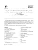
A total of ten variants of the devices were examined, as summarized in Table 1 and illustrated in Fig. 1. The key distinguishing
factor between these designs was the nature of the 2 D area, either
being a uniform flat bed or consisting of 16 discrete channels separated by spacers. Two types of spacers were studied (i.e. 0.1 or
0.5 mm thickness) and all types had the same flow distributor
format composed of cylindrical channels with an internal diameter varying from 0.3 to 1.0 mm with 90◦ angle T-junctions. These


T. Adamopoulou et al. / J. Chromatogr. A 1598 (2019) 77–84

79

Fig. 1. Typical spatial 2D-LC device with 3 main parts, viz. the flow distributor for the second-dimension separation (2 D) mobile phase, the first-dimension separation (1 D)
channel and the second-dimension separation (2 D) area. The line in the 2 D space represents a control line used for data extraction. Figure A shows the geometry used in
types III and VI, B shows the geometry used in types I and IV, and C shows the geometry used in type X.

dimensions took into consideration the best-possible resolution of
the DLP 3D-printer used in this research.
Simulations were conducted for both an empty 1 D channel and
for a 1 D channel containing a stationary-phase material. The porous
zone is not physically present and in order to approximate its effect
the superficial-velocity porous formulation is applied, where the
mixture velocities are calculated based on the flow rate in a porous
region. The porosity is assumed to be isotropic and porosity is not
taken into account for the calculation of diffusion terms in the transport equations. The examined types with an empty 1 D channel
are representative of 2D separation devices previously reported in
literature, in which isoelectric focusing was used as the 1 D separation method [31,32]. The types simulated for a 1 D channel with a
stationary phase represented the presence of an organic polymer
monolith. This presence was mimicked by treating the 1 D channel as a porous zone with permeability 1.7 10−13 m2 , a typical
value for polymer monoliths [33]. The dimensions of the 1 D channel were 24 × 1.5 × 1.5 mm (L × w × h). The process of 1 D injection
was not included in this study to eliminate any variations caused
by the 1 D injection and to reduce the computational cost. Instead, a
fully-filled 1 D channel was imposed during the initialization step,
containing a mixture of 1% (w/w) dye in water. For the 2 D simulations, water was introduced through the flow distributor. During
the transfer to the 2 D, the 1 D inlet and outlet were closed. The inlet
boundary condition was adjusted in all three types to achieve an
average velocity of 0.98 mm/s in the 2 D area. The dimensions of
the 2 D area were 24 × 10 × 1.5 mm (L × w × h) for the cases without
spacers, 23.5 × 10 × 1.5 mm (L × w × h) for the cases with spacers of
0.5 mm thickness and 23.9 × 10 × 1.5 mm (L × w × h) for the cases

with spacers of 0.1 mm thickness.
To determine the suitability of the design related to the spacer
thickness in the 2 D area, the method of moments was used to calculate the band variance. The calculation of the moments and variance
is reflected by Eqs. (1)–(4).
∞

(0) =

c (x) dx

(1)

0
∞

’(1) =

0

’(2) =

0

(0)
∞

2

=

’

xc (x) dx

x2 c (x) dx
(0)

(2) −

’(1)2

(2)

(3)
(4)

In Eqs. (1)–(4), (0) is the zeroth, ’(1) the first and ’(2) the
second moment, 2 is the variance and c(x) corresponds to the
transversally averaged concentration of dye across the 2 D zone

Fig. 2. Photographs of 3D-printed devices used for assessing flow profiles. Devices of
type X (left), type XI (middle) and type XII (right) without stationary-phase material.

from x to x + dx as calculated per time step. In this way, the transfer of the analytes from the 1 D channel to the 2 D area could be
observed. During the grid independence study the maximum difference for pressure and for the velocity component of the direction
of the flow was 0.0023% and 0.0021%, respectively. The time-step
choice was made in respect with the minimum cell volume and the
chosen velocity.
2.3. 3D-Printing of microfluidic devices
Microfluidic devices were designed using SOLIDWORKS (Dassault Systèmes SOLIDWORKS, Waltham, MA, USA) and Autodesk

Inventor (Autodesk, San Rafael, CA, USA). Devices (Fig. 2; vide infra
Figs. 6 and 8) were fabricated through digital light processing
(DLP) using an Asiga Pico 2 HD 3D-printer (Asiga Germany, Erfurt,
Germany).
The design was converted to STL format, loaded through the 3D
printer software interface (Asiga Composer), and printing orientation and settings were optimized for high resolution and fabrication
time The devices shown in Fig. 2 were printed vertically to the build
platform of the printer, while the devices used for pressure testing
(Fig. 8) were printed horizontally to the build platform. This placement difference had an effect on the appearance of the devices
where in Fig. 2 the devices have a “milky” appearance while the
top layer of the device in Fig. 8 is more shiny. After 3D-printing,
devices were post-processed by sonication and flushing of channels with 2-propanol and nitrogen gas to remove any uncured resin.
Finally, parts were placed in a Pico Flash UV chamber (type 87 DR301C, 36 W, 365 nm; 3DXS, Erfurt, Germany) and cured for 30 min.
To make the devices connectable, straight threads (#10-32 UNC,


80

T. Adamopoulou et al. / J. Chromatogr. A 1598 (2019) 77–84

Fig. 3. Relative dye concentration (A&B) recorded at a control plane close to the transition zone (3 mm from the 1 D to 2 D interface zone towards the 2 D outlet) and band
variance along the 2 D direction (C&D) for devices with an empty 1 D channel, i.e. type I-III (A&C) and for devices with a 1 D channel with a stationary phase i.e. types IV–VI
(B&D). Solid line corresponds to the flat-bed 2 D area, dotted line to 2 D channels with 0.1 mm spacer thickness, and dashed line corresponds to 2 D channels with 0.5 mm
spacer thickness.

major diameter 4.83 mm, 95 thread pitch 0.794 mm) were created
using a hand tap. A conical ferrule seat was 3D-printed to facilitate
a leak-proof connection to the outlet of the device.

pressure was recorded. All measurements were conducted (at least)

in triplicates. Appropriate safety measures were taken to shield
analysts from any possible spray of liquid or flying pieces of resin.
Neither of these latter were encountered during the study.

2.4. Evaluation of printed devices
3. Results and discussion
To compare the performance in terms of dye flow profiles and
band-broadening effects between simulated and printed devices,
flow tests were conducted in printed devices that featured a flow
distributor, a 1 D channel, a 2 D area and a flow collector. The devices
were completely filled with 2-propanol and a mixture of red dye
dissolved in 2-propanol (1%) was then injected through the distributor for flow visualization. The injection was realized with an
injection valve, and the injection volume was less than 5% of the volume of the 2 D area. Flow profiles were recorded with a Canon EOS
1300D camera (Canon Inc., Tokyo, Japan). To quantitatively evaluate the performance of the devices, the red colour intensity was
quantified along two horizontal (1 D direction) control lines at the
beginning and end of the 2 D area and analysis was conducted using
Mathematica (Wolfram, Champaign, IL, USA). Finally, the pressure
limit of the printed devices was studied by increasing the flow rate
until failure (i.e. breakage or leakage). For this purpose, devices with
a flow distributor, an empty flat 2 D area and inlet and outlet connections were printed. Devices were connected to an LC-10 AD VP
Shimadzu liquid-chromatography pump (Shimadzu, Kyoto, Japan)
and the flow rate was gradually increased until failure while the

Various design aspects, which were thought to affect the performance of spatial two-dimensional liquid-chromatography devices,
were assessed. As shown in Fig. 1, the examined devices consisted
of three main parts, viz. (i) the flow distributor aimed to homogeneously distribute the mobile phase for the second-dimension (2 D)
separation across (ii) the first-dimension (1 D) separation channel
and (iii) the 2 D separation area (i.e. flat bed or 16 discrete channels). A separation in the described devices occurs by the following
series of subsequent steps, viz. (i) sample injection and 1 D separation, while the 2 D inlet and outlet are closed, (ii) introduction of
the mobile phase for the 2 D separation, while the 1 D inlet and outlet are closed, (iii) transfer of analytes from the 1 D channel to the

2 D area, and finally (iv) parallel separation of the entire content of
the 1 D channel in the 2 D area. Detection can occur either in-situ
(e.g. by confocal spectroscopy in a transparent device), on-line at
the end of the 2 D area (e.g. by laser-induced fluorescence, LIF [19]),
or offline via collection of the effluent (e.g. by immobilization on a
substrate followed by matrix-assisted laser-desorption/ionization
mass spectrometry, MALDI-MS [31]).


T. Adamopoulou et al. / J. Chromatogr. A 1598 (2019) 77–84

81

Fig. 4. Contour plots of mass fraction of dye in type II (left) and type V (right) devices after the 2 D injection of water for one device volume. Colour scale ranges from 0 (blue)
to 9.89 10−3 (red) (For interpretation of the references to colour in this figure legend, the reader is referred to the web version of this article).

3.1. Computational fluid dynamics
3.1.1. Effect of 2 D geometry on band broadening
The first six device types described in Table 1 were compared
in terms of band variance and relative dye concentration during
transfer of dye from the 1 D channel to the 2 D area. In all types the
initial state was a 1 D channel uniformly filled with a mixture of dye
and water. Subsequently, water was introduced through the flow
distributor, while the 1 D inlet and outlet were closed. As a result,
the dye mixture in the 1 D channel was transferred to the 2 D area.
The relative dye concentration and the band variance recorded
over time are shown in Fig. 3. Fig. 3A and B depict the band profiles
recorded at a control plane close to the transition zone (3 mm from
the 1 D to 2 D interface zone towards the 2 D outlet) for types I-III,
with an empty 1 D channel, and types IV-VI, with a 1 D channel containing a stationary material, respectively. The open 1 D channels

give rise to an initial sharp band, followed by a seemingly endless
tail, indicative of the presence of stagnant areas in between flow
lines from the distributor to the 2 D area. In case where stationary material is present in the 1 D channel the initial pulse is a bit
broader, but all of the dye is washed from the 1 D channel within a
few seconds. The corresponding band variances in the 2 D direction,
calculated using Eqs. (1)–(4), are much higher (app. hundred-fold)
in cases where there is no 1 D stationary-phase material (Fig. 3C)
than in case of a 1 D channel containing a stationary-phase material (Fig. 3D). In case of an empty 1 D channel the band variance
keeps increasing during the 2 D injection of one device volume,
while it levels off in case of a 1 D channel containing a stationary
material.
In Fig. 3A it can be observed that for the device types with an
empty 1 D channel (types I–III) the dye concentration at the control
plane remains significant, long after the band has moved towards
the outlet. This implies that the dye remains present in the device
after the transfer operation is meant to have ended. This is in accordance with the contour plot shown in Fig. 4 (left), where dye is
seen to have remained in the 1 D channel after a full device volume
of water has been flushed through. This incomplete dye transfer indicates poorly-permeated (“dead”) zones in the 1 D channel.
When comparing types containing stationary material in the 1 D
channel (types IV-VI), it is interesting to note that types IV and
VI, which represent a flat-bed 2 D area and one with discrete 2 D
channels with the minimal 0.1 mm spacer thickness, respectively,
show an almost identical, symmetrical dye-concentration profile.
On the other hand, type V, which features discrete 2 D channels
with 0.5 mm spacer thickness, gives rise to a broader, tailing dye-

concentration profile, due to dead zones formed in front of these
spacers.
3.1.2. Analyte transfer from 1 D channel to 2 D separation spaces
Fig. 4shows two examples of the dye plugs migrating to the end

of the 2 D area for the type II (empty 1 D channel, discrete 2 D channels
with 0.5 mm spacer thickness) and type V (1 D channel with stationary material, discrete 2 D channels with 0.5 mm spacer thickness)
devices.
To study the issue of incomplete transfer of dye from the 1 D
channel to the 2 D area caused by poorly-permeated zones in case
of an empty 1 D channel, the effect of the internal diameter of the
bifurcating distributor channels (i.e. 0.3, 0.6, 0.7, 0.8, and 1.0 mm) on
the dye transfer was examined. Increasing the distributor channel
diameter might decrease the size of the dead zones located in the
1 D channel between the distributor entry points. Types II and VII-X
with an empty 1 D channel and a 2 D area consisting of discrete channels with 0.5 mm spacer thickness were selected for this study. The
height and width of the 1 D channels (both 1.5 mm) and the height
and width of the 2 D channels (1.5 mm and 1.0 mm, respectively),
where kept constant in this study.
Fig. 5 A shows a histogram of the volume fractions of the binned
mesh elements relative to the total 1 D channel volume based on the
velocity magnitude from steady-state simulations on the device.
Low local velocities indicate poorly-permeated dead zones in the
1 D channel. It is seen that narrow flow distributor channels cause
dead zones in more than 10% of the total volume (left-hand side of
Fig. 5A) and would therefore cause poor analyte transfer. Increasing
the internal diameter clearly reduces the volume fraction of nearstagnant zones. The latter can be understood from the fact that
the wider flow distributor channels lead to a larger fraction of 1 D
channel that is readily swept by the incoming 2 D flow distributor
flow.
Transient simulations mimicking analyte transfer with a dye
flushed into the 2 D space were performed. In Fig. 5B the dye recovery after the band has transferred from the 1 D channel to the 2 D
channels is shown. Ideally, 100% of the dye is recovered, but thus
ideal situation is never reached because of the dead zones in the 1 D
channel. The percentage of dye remaining in the 1 D channel is seen

to decrease when the diameter of the distributor channel diameter increases from 0.3 to 1.0 mm. This is in accordance with the
reduction of the dead zones observed in Fig. 5A. These results confirm the trends seen with the steady-state simulations (Fig. 5A), i.e.
that larger diameter distributor channels facilitate better analyte
transfer between the two dimensions.


82

T. Adamopoulou et al. / J. Chromatogr. A 1598 (2019) 77–84

Fig. 5. A) Velocity distribution within the 1 D channel during transfer from the 1 D channel to 2 D region. The vertical axis displays the fraction of the total volume that exhibits
a specific local velocity magnitude during a 2 D flushing step with a bin size of 5 ␮m for device types II, VII-X (solid lines) with empty 1 D channel and V (dashed line) with a
1
D channel with stationary-phase material. B) Calculated recovery of the dye solution at the 2 D outlet measured after flushing with one total device volume.

Fig. 6. Photographs of 3D-printed devices during flow testing, after the dye started entering the 2 D space. Devices of type X (left), type XII (middle) and type XI (right) without
stationary-phase material.

Nevertheless, transferring under 90% of the analytes to the
second-dimension region is far from ideal for effective 2D-LC separations. This can be mitigated by the presence of a stationary
phase in the 1 D region, as illustrated in Figs. 4 and 5. As can
be observed from case 0.3 P in Fig. 5, which incorporates a 0.3mm flow-distributor and a porous 1 D channel, the flow resistance
caused by the stationary phase (5.6 1012 m−2 ) homogenizes the
flow profile in the y-direction and results in a nearly complete (up to
99.8%) transfer to the 2 D space. However, a microfluidic device containing two different stationary phases can introduce a new set of
practical challenges, such as analyte spill-over between the stationary phases. Therefore, novel analyte transfer solutions such as the
Twist valve [34] may be necessary for achieving sufficient analyte
transfer and consequently, high peak-capacities in spatial 2D-LC
devices.

points was then subtracted from the variance at the points near
the end of the 2 D area. In Fig. 7A when observing only the variance
calculated at the starting points the highest value corresponds to
the type with discrete channels with 0.5 mm spacer thickness and
the lowest to the case with no spacers. In Fig. 7B, the difference in
variance between the two control lines per point is presented, with
the largest contribution to band variance observed in the type with
discrete channels with 0.1 mm spacer thickness, followed by the
type with discrete channels with 0.5 mm spacer thickness, while
the flat bed had the lowest contribution to band variance.
When the printed device with the 0.1 mm thick spacers was cut
open and inspected, it was observed that the spacers were not completely straight. This imperfection is suspected to be the cause of
the discrepancy between computational and experimental testing.
More extensive experimentation with different designs and possibly different 3D-printing techniques will be required to advance
the technology.

3.2. Experimental evaluation of 3D-Printed microfluidic devices
3.2.1. Flow profiles
After comparing a variety of microfluidic devices using CFD, a
selection of devices was prototyped by high-resolution DLP 3Dprinting. To study the effect of the 2 D geometries on flow profiles
in the 3D-printed devices, a dye mixture was injected to the three
examined types, as it is shown in Fig. 6 viz. a flat (undivided) 2 D bed
and two types with discrete channels in the 2 D area. A drawing of
the details of the in- and outlets to the 1 D channel has been added
to the supplementary material (Fig. S1). This shows significant dead
zones can be expected to develop, explaining (at least partly) the
relatively wide zone injected in the 2 D in Fig. 6.
The band variance was calculated at 16 equidistant control
points along two control lines parallel to the 1 D channel, one at the
start and one at the end of the 2 D area. The variance at the starting

3.2.2. Pressure limit of the devices
In pressure-driven liquid chromatography, a high-pressure
resistance is desired for successful operation of a device. For our
printed devices (Fig. 8) we aimed to determine the weakest points
in the design (i.e. the points most prone to failure) and the pressure
at failure in relation to the wall thickness. An initial encasing with
wall thickness of 2 mm was chosen. In this case the device appeared
most vulnerable near the outlet connection and the pressure at
failure was about 1 MPa.
An increase of the encasing thickness to 5 mm was then realized, with the wall covering the surface of the outlet connector. The
flow rate in the devices was raised step-wise until failure or up to a
flow rate of 3 mL/min. The average maximum pressure was 3.5 MPa.
In the majority of tests failure of the device was not encountered,


T. Adamopoulou et al. / J. Chromatogr. A 1598 (2019) 77–84

83

Fig. 7. A) Variance at the starting control line per point. B) Difference in variance between the ending and starting control lines per point. Black corresponds to the case with
no spacers in the 2 D, grey to the case with spacers of 0.5 mm thickness and light grey to the case with spacers of 0.1 mm thickness.

Fig. 8. Device used during pressure testing, consisting of a distributor, a flat bed and an outlet connector. In this case the top and bottom wall-thickness of 5 mm is used.

apart from the method with the steepest increase (increment of
1.5 mL/min instead of 1 mL/min in other cases), in which case failure occurred at approximately 4.5 MPa. However, some leakage
around the connections was present in the majority of the cases
at pressures exceeding 3 MPa.
The pressure tests indicate that the devices printed with a regular commercial photopolymer (i.e. not designed for maximal tensile

strength) can operate at moderate pressures. High pressures used
in column-based HPLC and UHPLC are not necessary for achieving
high peak capacities spatial multi-dimensional separation [22]. If
necessary, the pressure limit of the chips can be increased by using
thicker walls, other photopolymers or external structural supports
for the device. However, these results point to the ongoing challenge of developing pressure-resistant, low-dispersion fittings to
3D-printed polymer devices.
4. Conclusion and outlook
Two aspects of prospective two-dimensional spatial separation
devices were studied, viz. efficient analyte transfer from the first
(1 D) to the second (2 D) dimension and band broadening in the
2 D area of the device. Ten types of devices were studied using
computational fluid dynamics (CFD) and initial experiments were
performed on a selection of devices.
The presence of a stationary phase in the 1 D channel was found
to have a dramatic effect on the efficiency of analyte transfer from
1 D to 2 D. Without a stationary-phase material present, a significant
amount of the dye used to mimic analytes present in the 1 D channel remained in near-stagnant dead zones long after transfer was
meant to be completed. As a result, injection bands in the second

dimension showed a high variance and excessive tailing. To further
explore the effects of dead zones in 1 D channels without a stationary material present, the diameter of the channels in the 2 D flow
distributor was varied. Analyte losses were found to decrease upon
increasing the diameter of the distributor flow channels.
CFD calculations suggested that the presence of spacers in the
2 D area would increase band dispersion. In the case of a 1 D channel
with stationary material present, the 2 D band dispersion was found
to increase with increasing spacer thickness, while in the cases with
an empty 1 D channel this trend was not observed.
The contributions of spacers to the band dispersion in the 2 D

area and the pressure limit of the fabricated devices were studied
experimentally in devices created by high-resolution 3D-printing.
A design without spacers was found to exhibit the lowest variance,
in accordance with the CFD study. Thick (0.5 mm) spacers were
found to perform better than thin (0.1 mm spacers), but this may
be due to imperfections in the printed devices. Understandably,
the thickness of the encasing of devices was found to significantly
affect the pressure limit of 3D-printed devices. When increasing
the encasing thickness from 2 mm to 5 mm the pressure at failure
was found to increase from 1 to 4.5 MPa, although some leakage was observed around the connectors at pressures of about
3 MPa. The pressure limit may be improved with the use of an
external holder and improved connectors will need to be studied.
The present study has contributed to progress in twodimensional spatial chromatography. Suitable devices can, in
principle, be created using 3D-printing and the knowledge created in the present study should contribute to the realization of
successful devices in the near future.


84

T. Adamopoulou et al. / J. Chromatogr. A 1598 (2019) 77–84

Acknowledgements
The authors would like to acknowledge Noor Abdulhussain for
her contributions to the pressure testing, Liana S. Roca for her assistance during flow testing and Bob W.J. Pirok and Alan Rodrigo
García Cicourel for assisting in organizing the necessary laboratory
equipment for the realization of the flow tests.
The STAMP project is funded under Horizon 2020-Excellent
Science-European Research Council (ERC), Project 694151. The sole
responsibility of this publication lies with the authors. The European Union is not responsible for any use that may be made of the
information contained therein.

Sander Deridder gratefully acknowledges a research grant from
the Research Foundation – Flanders (FWO-Vlaanderen).
Appendix A. Supplementary data
Supplementary material related to this article can be found, in
the online version, at doi: />03.041.
References
[1] B.W.J. Pirok, D.R. Stoll, P.J. Schoenmakers, Recent developments in
two-dimensional liquid chromatography – fundamental improvements for
practical applications, Anal. Chem. 91 (2018) 240–263, />1021/acs.analchem.8b04841.
[2] M. Gao, D. Qi, P. Zhang, C. Deng, X. Zhang, Development of multidimensional
liquid chromatography and application in proteomic analysis, Expert Rev.
Proteom. 7 (2010) 665–678, />[3] A. D’Attoma, S. Heinisch, On-line comprehensive two dimensional
separations of charged compounds using reversed-phase high performance
liquid chromatography and hydrophilic interaction chromatography. Part II:
application to the separation of peptides, J. Chromatogr. A 1306 (2013) 27–36,
/>[4] X. Zhang, A. Fang, C.P. Riley, M. Wang, F.E. Regnier, C. Buck, Multi-dimensional
liquid chromatography in proteomics-a review, Anal. Chim. Acta 664 (2010)
101–113, />[5] A. Van Der Horst, P.J. Schoenmakers, Comprehensive two-dimensional liquid
chromatography of polymers, J. Chromatogr. A 1000 (2003) 693–709, http://
dx.doi.org/10.1016/S0021-9673(03)00495-3.
[6] P. Schoenmakers, P. Aarnoutse, Multi-dimensional separations of polymers,
Anal. Chem. 86 (2014) 6172–6179, />[7] E. Uliyanchenko, S. Van Der Wal, P.J. Schoenmakers, Challenges in polymer
analysis by liquid chromatography, Polym. Chem. 3 (2012) 2313, http://dx.
doi.org/10.1039/c2py20274c.
[8] T. Beelders, K.M. Kalili, E. Joubert, D. de Beer, A. de Villiers, Comprehensive
two-dimensional liquid chromatographic analysis of rooibos (Aspalathus
linearis) phenolics, J. Sep. Sci. 35 (2012) 1808–1820, />1002/jssc.201200060.
[9] K.M. Kalili, A. de Villiers, Off-line comprehensive two-dimensional
hydrophilic interaction x reversed phase liquid chromatographic analysis of
green tea phenolics, J. Sep. Sci. 33 (2010) 853–863, />jssc.200900673.

[10] C.M. Willemse, M.A. Stander, J. Vestner, A.G.J. Tredoux, A. De Villiers,
Comprehensive two-dimensional hydrophilic interaction chromatography
(HILIC) × reversed-phase liquid chromatography coupled to high-resolution
mass spectrometry (RP-LC-UV-MS) analysis of anthocyanins and derived
pigments in red wine, Anal. Chem. 87 (2015) 12006–12015, />10.1021/acs.analchem.5b03615.
[11] X. Ouyang, P. Leonards, J. Legler, R. van der Oost, J. de Boer, M. Lamoree,
Comprehensive two-dimensional liquid chromatography coupled to high
resolution time of flight mass spectrometry for chemical characterization of
sewage treatment plant effluents, J. Chromatogr. A 1380 (2015) 139–145,
/>[12] B.W.J. Pirok, A.F.G. Gargano, P.J. Schoenmakers, Optimizing separations in
on-line comprehensive two-dimensional liquid chromatography, J. Sep. Sci.
41 (2017) 68–98, />
[13] J.C. Giddings, Sample dimensionality: a predictor of order-disorder in
component peak distribution in multidimensional separation, J. Chromatogr.
A. 703 (1995) 3–15, />[14] G. Groeneveld, M.N. Dunkle, M. Rinken, A.F.G. Gargano, A. de Niet, M. Pursch,
E.P.C. Mes, P.J. Schoenmakers, Characterization of complex polyether polyols
using comprehensive two-dimensional liquid chromatography hyphenated to
high-resolution mass spectrometry, J. Chromatogr. A 1569 (2018) 128–138,
/>[15] G. Guiochon, M.F. Gonnord, A. Siouffi, M. Zakaria, Study of the performances
of thin-layer chromatography. VII. Spot capacity in two-dimensional
thin-layer chromatography, J. Chromatogr. A. 250 (1982) 1–20, .
org/10.1016/S0021-9673(00)95205-1.
[16] J.C. Giddings, Two-dimensional separations: concept and promise, Anal.
Chem. 56 (2007) 1258A–1270A, />[17] K.S. Mriziq, G. Guiochon, Column properties and flow profiles of a flat, wide
column for high-pressure liquid chromatography, J. Chromatogr. A 1187
(2008) 180–187, />[18] G. Guiochon, N. Marchetti, K. Mriziq, R.A. Shalliker, Implementations of
two-dimensional liquid chromatography, J. Chromatogr. A 1189 (2008)
109–168, />[19] C. Das, J. Zhang, N.D. Denslow, Z.H. Fan, Integration of isoelectric focusing
with multi-channel gel electrophoresis by using microfluidic pseudo-valves,
Lab Chip 7 (2007) 1806–1812, />[20] J. Liu, S. Yang, C.S. Lee, D.L. DeVoe, Polyacrylamide gel plugs enabling 2-D

microfluidic protein separations via isoelectric focusing and multiplexed
sodium dodecyl sulfate gel electrophoresis, Electrophoresis 29 (2008)
2241–2250, />[21] G. Guiochon, L.A. Beaver, M.F. Gonnord, A.M. Siouffi, M. Zakaria, Theoretical
investigation of the potentialities of the use of a multidimensional column in
chromatography, J. Chromatogr. A 255 (1983) 415–437, />1016/S0021-9673(01)88298-4.
[22] E. Davydova, P.J. Schoenmakers, G. Vivó-Truyols, Study on the performance of
different types of three-dimensional chromatographic systems, J. Chromatogr.
A 1271 (2013) 137–143, />[23] B. Wouters, E. Davydova, S. Wouters, G. Vivo-Truyols, P.J. Schoenmakers, S.
Eeltink, Towards ultra-high peak capacities and peak-production rates using
spatial three-dimensional liquid chromatography, Lab Chip. 15 (2015)
4415–4422, />[24] J.P. Grinias, R.T. Kennedy, Trends in analytical chemistry advances in and
prospects of microchip liquid chromatography, Trends Anal. Chem. 81 (2016)
110–117, />[25] E. Davydova, S. Wouters, S. Deridder, G. Desmet, S. Eeltink, P.J. Schoenmakers,
Design and evaluation of microfluidic devices for two-dimensional spatial
separations, J. Chromatogr. A 1434 (2016) 127–135, />1016/j.chroma.2016.01.003.
[26] E. Davydova, S. Deridder, S. Eeltink, G. Desmet, P.J. Schoenmakers,
Optimization and evaluation of radially interconnected versus bifurcating
flow distributors using computational fluid dynamics modelling, J.
Chromatogr. A 1380 (2015) 88–95, />12.063.
[27] S. Jespers, S. Deridder, G. Desmet, A microfluidic distributor combining
minimal volume, minimal dispersion and minimal sensitivity to clogging, J.
Chromatogr. A 1537 (2018) 75–82, />01.029.
[28] H.K. Versteeg, W. Malalasekra, An Introduction to Computational Fluid
Dynamics: the Finite Volume Method, Pearson Education Ltd., Harlow,
England, 2007.
[29] R. Taylor, R. Krishna, Multicomponent Mass Transfer, Wiley, 1993.
[30] P. Gzil, N. Vervoort, G.V. Baron, G. Desmet, Advantages of perfectly ordered
2-D porous pillar arrays over packed bed columns for LC separations: a
theoretical analysis, Anal Chem. 75 (2003) 6244–6250, />1021/ac034345m.
[31] J. Liu, C.F. Chen, S. Yang, C.C. Chang, D.L. DeVoe, Mixed-mode electrokinetic

and chromatographic peptide separations in a microvalve-integrated polymer
chip, Lab Chip 10 (2010) 2122–2129, />[32] B. Wouters, J. De Vos, G. Desmet, H. Terryn, P.J. Schoenmakers, S. Eeltink,
Design of a microfluidic device for comprehensive spatial two-dimensional
liquid chromatography, J. Sep. Sci. 38 (2015) 1123–1129.
[33] S. Deridder, S. Eeltink, G. Desmet, Computational study of the relationship
between the flow resistance and the microscopic structure of polymer
monoliths, J. Sep. Sci. 34 (2011) 2038–2046, />201100220.
[34] T. Adamopoulou, S. Deridder, G. Desmet, P.J. Schoenmakers, Two-dimensional
insertable separation tool (twist) for flow confinement in spatial separations,
J. Chromatogr. A 1577 (2018) 120–123, />2018.09.054.