Báo cáo khoa học: "Recognizing Textual Parallelisms with edit distance and similarity degree" docx
Bạn đang xem bản rút gọn của tài liệu. Xem và tải ngay bản đầy đủ của tài liệu tại đây (230.16 KB, 8 trang )
Recognizing Textual Parallelisms with edit distance and similarity degree
Marie Gu
´
egan and Nicolas Hernandez
LIMSI-CNRS
Universit´e de Paris-Sud, France
|
Abstract
Detection of discourse structure is crucial
in many text-based applications. This pa-
per presents an original framework for de-
scribing textual parallelism which allows
us to generalize various discourse phe-
nomena and to propose a unique method
to recognize them. With this prospect, we
discuss several m ethods in order to iden-
tify the most appropriate one for the prob-
lem, and evaluate them based on a manu-
ally annotated corpus.
1 Introduction
Detection of discourse structure is crucial in many
text-based applications such as Information Re-
trieval, Question-Answering, Text Browsing, etc.
Thanks to a discourse structure one can precisely
point out an information, provide it a local context,
situate it globally, link it to others.
The context of our research is to improve au-
tomatic discourse analysis. A key feature of the
most popular discourse theories (RST (Mann and
Thompson, 1987), SDRT (Asher, 1993), etc.) is
the distinction between two sorts of discourse re-
lations or rhetorical functions: the subordinating
and the coordinating relations (some parts of a
text play a subordinate role relative to other parts,
while some others have equal importance).
In this paper, we focus our attention on a dis-
course feature we assume supporting coordination
relations, namely the Textual Parallelism. Based
on psycholinguistics studies (Dubey et al., 2005),
our intuition is that similarities concerning the sur-
face, the content and the structure of textual units
can be a way for authors to explicit their intention
to consider these units with the same rhetorical im-
portance.
Parallelism can be encountered in many specific
discourse structures such as continuity in infor-
mation structure (Kruijff-Korbayov´a and Kruijff,
1996), frame structures (Charolles, 1997), VP el-
lipses (Hobbs and Kehler, 1997), headings (Sum-
mers, 1998), enumerations (Luc et al., 1999), etc.
These phenomena are usually treated mostly inde-
pendently within individual systems with ad-hoc
resource developments.
In this work, we argue that, depending on de-
scription granularity we can proceed, computing
syntagmatic (succession axis of linguistic units)
and paradigmatic (substitution axis) similarities
between units can allow us to generically handle
such discourse structural phenomena. Section 2
introduces the discourse parallelism phenomenon.
Section 3 develops three methods we implemented
to detect it: a similarity degree measure, a string
editing distance (Wagner and Fischer, 1974) and a
tree editing distance
1
(Zhang and Shasha, 1989).
Section 4 discusses and evaluates these methods
and their relevance. The final section reviews re-
lated work.
2 Textual parallelis m
Our notion of parallelism is based on similarities
between syntagmatic and paradigmatic represen-
tations of (constituents of) textual units. These
similarities concern various dimensions from shal-
low to deeper description: layout, typography,
morphology, lexicon, syntax, and semantics. This
account is not limited to the semantic dimension
as defined by (Hobbs and Kehler, 1997) who con-
sider text fragments as parallel if the same predi-
cate can be inferred from them with coreferential
or similar pairs of arguments.
1
For all measures, elementary units considered are syn-
tactic tags and word tokens.
281
We observe parallelism at various structural lev-
els of text: among heading structures, VP ellipses
and others, enumerations of noun phrases in a
sentence, enumerations with or without markers
such as frame introducers (e.g. “In France, . . . In
Italy, . . . ”) or typographical and layout markers.
The underlying assumption is that parallelism be-
tween some textual units accounts for a rhetorical
coordination relation. It means that these units can
be regarded as equally important.
By describing textual units in a two-tier frame-
work composed of a paradigmatic level and syn-
tagmatic level, we argue that, depending on the
description granularity we consider (potentially at
the character level for item numbering), we can
detect a wide variety of parallelism phenomena.
Among parallelism properties, we note that the
parallelism of a given number of textual units is
based on the parallelism of their constituents. We
also note that certain semantic classes of con-
stituents, such as item numbering, are more effec-
tive in marking parallelism than others.
2.1 An example of parallelism
The following example is extracted from our cor-
pus (see section 4.1). In this case, we have an enu-
meration without explicit markers.
For the purposes of chaining, each type of link
between WordNet synsets is assigned a direction
of up, down, or horizontal.
Upward links correspond to generalization: for
example, an upward link from apple to fruit indi-
cates that fruit is more general than apple.
Downward links correspond to specialization:
for example, a link from fruit to apple would have
a downward direction.
Horizontal links are very specific specializations.
The parallelism pattern of the first two items is de-
scribed as follows:
[JJ + suff =ward] links correspond to [NN + suff
= alization] : for example , X link from Y to Z .
This pattern indicates that several item con-
stituents can be concerned by parallelism and that
similarities can be observed at the typographic,
lexical and syntactic description levels. Tokens
(words or punctuation marks) having identical
shallow descriptions are written in italics. The
X, Y and Z variables stand for matching any non-
parallel text areas between contiguous parallel tex-
tual units. Some words are parallel based on
their syntactic category (“JJ” / adjectives, “NN” /
nouns) or suffix specifications (“suff” attribute).
The third item is similar to the first two items but
with a simpler pattern:
JJ links U [NN + suff =alization] W .
Parallelism is distinguished by these types of sim-
ilarities between sentences.
3 Methods
Three methods were used in this study. Given a
pair of sentences, they all produce a score of sim-
ilarity between these sentences. We first present
the preprocessing to be performed on the texts.
3.1 Prior processing applied on the texts
The texts were automatically cut into sentences.
The first two steps hereinafter have been applied
for all the methods. The last third was not applied
for the tree editing distance (see 3.3). Punctua-
tion marks and syntactic labels were henceforward
considered as words.
1. Text homogenization: lemmatization together
with a semantic standardization. Lexical chains
are built using WordNet relations, then words are
replaced by their most representative synonym:
Horizontal links are specific specializations.
horizontal connection be specific specialization .
2. Syntactic analysis by (Charniak, 1997)’s parser:
( S1 ( S ( NP ( JJ Horizontal ) (NNS links ) ( VP
( AUX are) ( NP ( ADJP ( JJ specific ) ( NNS
specializations ) ( SENT .)))))))
3. Syntactic structure flattening:
S1 S NP JJ Horizontal NNS links VP AUX are
NP ADJP JJ specific NNS specializations SENT.
3.2 Wagner & Fischer’s string edit distance
This method is based on Wagner & Fischer’s
string edit distance algorithm (Wagner and Fis-
cher, 1974), applied to sentences viewed as strings
of words. It computes a sentence edit distance, us-
ing edit operations on these elementary entities.
The idea is to use edit operations to transform
sentence S
1
into S
2
. Similarly to (Wagner and Fis-
cher, 1974), we considered three edit operations:
1. replacing word x ∈ S
1
by y ∈ S
2
: (x → y)
2. deleting word x ∈ S
1
: (x → λ)
3. inserting word y ∈ S
2
into S
1
: (λ → y)
By definition, the cost of a sequence of edit op-
erations is the sum of the costs
2
of the elementary
2
We used unitary costs in this study
282
operations, and the distance between S
1
and S
2
is
the cost of the least cost transformation of S
1
into
S
2
. Wagner & Fischer’s method provides a simple
and effective way (O(|S
1
||S
2
|)) to compute it. To
reduce size effects, we normalized by
|S
1
|+|S
2
|
2
.
3.3 Zhang & Shasha’s algorithm
Zhang & Shasha’s method (Zhang and S hasha,
1989; Dulucq and Tichit, 2003) generalizes Wag-
ner & Fischer’s edit distance to trees: given two
trees T
1
and T
2
, it computes the least-cost se-
quence of edit operations that transforms T
1
into
T
2
. Elementary operations have unitary costs and
apply to nodes (labels and words in the syntactic
trees). These operations are depicted below: sub-
stitution of node c by node g (top figure), inser-
tion of node d (middle fig.), and deletion of node
d (bottom fig.), each read from left to right.
Tree edit distance d(T
1
, T
2
) is determined after
a series of intermediate calculations involving spe-
cial subtrees of T
1
and T
2
, rooted in keyroots.
3.3.1 Keyroots, special subtrees and forests
Given a certain node x, L(x) denotes its left-
most leaf descendant. L is an equivalence rela-
tion over nodes and keyroots (KR) are by definition
the equivalence relation representatives of high-
est postfix index. Special subtrees (SST) are the
subtrees rooted in these keyroots. Consider a tree
T postfix indexed (left figure hereinafter) and its
three SSTs (right figure).
SST(k
1
) rooted in k
1
is denoted:
T [L(k
1
), L(k
1
) + 1, . . . , k
1
]. E.g: SST(3) =
T [1, 2, 3] is the subtree containing nodes a, b, d.
A forest of SST(k
1
) is defined as:
T [L(k
1
), L(k
1
) + 1, . . . , x], where x is a
node of SST(k
1
). E.g: SST(3) has 3 forests :
T [1] (node a), T [1, 2] (nodes a and b) and itself.
Forests are ordered sequences of subtrees.
3.3.2 An idea of how it works
The algorithm computes the distance between all
pairs of SSTs taken in T
1
and T
2
, rooted in
increasingly-indexed keyroots. In the end, the last
SSTs being the full trees, we have d(T
1
, T
2
).
In the main routine, an N
1
× N
2
array called
TREED IST is progressively filled with values
TREED IST(i, j) equal to the distance between the
subtree rooted in T
1
’s i
th
node and the subtree
rooted in T
2
’s j
th
node. The bottom right-hand
cell of TREEDIST is therefore equal to d(T
1
, T
2
).
Each step of the algorithm determines the edit
distance between two SSTs rooted in keyroots
(k
1
, k
2
) ∈ (T
1
× T
2
). An array FDIST is ini-
tialized for this step and contains as many lines
and columns as the two given SSTs have nodes.
The array is progressively filled with the distances
between increasing forests of these SSTs, simi-
larly to Wagner & Fischer’s method. The bot-
tom right-hand value of FDIST contains the dis-
tance between the SSTs, which is then stored in
TREED IST in the appropriate cell. Calculations
in FDIST and TREEDIST rely on the double re-
currence formula depicted below:
The first formula is used to compute the dis-
tance between two forests (a white one and a black
one), each of which is composed of several trees.
The small circles stand for the nodes of highest
postfix index. Distance between two forests is de-
fined as the minimum cost operation between three
possibilities: replacing the rightmost white tree by
the rightmost black tree, deleting the white node,
or inserting the black node.
The second formula is analogous to the first one,
in the special case where the forests are reduced to
a single tree. The distance is defined as the mini-
mum cost operation between: replacing the white
node with the black node, deleting the white node,
or inserting the black node.
283
It is important to notice that the first formula
takes the left context of the considered subtrees
into account
3
: ancestor and left sibling orders are
preserved. It is not possible to replace the white
node with the black node directly, the whole sub-
tree rooted in the white node has to be replaced.
The good thing is, the cost of this operation has
already been computed and stored in TREEDIST.
Let’s see why all the computations required at a
given step of the recurrence formula have already
been calculated. Let two SSTs of T
1
and T
2
be
rooted in pos
1
and pos
2
. Considering the symme-
try of the problem, let’s only consider what hap-
pens with T
1
. When filling FDIST(pos1, pos
2
),
all nodes belonging to SST(pos
1
) are run through,
according to increasing postfix indexes. Consider
x ∈ T [L(pos
1
), . . . , pos
1
]:
If L(x) = L(pos
1
), then x belongs to the left-
most branch of T [L(pos
1
), . . . , pos
1
] and forest
T [L(pos
1
), . . . , x] is reduced to a single tree. By
construction, all FDIST(T [L(pos
1
), . . . , y], −) for
y ≤ x − 1 have already been computed. If things
are the same for the current node in SST(pos
2
),
then TREEDIST(T [L(pos
1
), . . . , x], −) can be
calculated directly, using the appropriate FDIST
values previously computed.
If L(x) = L(pos
1
), then x does not belong
to the leftmost branch of T [L(pos
1
), . . . , pos
1
]
and therefore x has a non-empty left context
T [L(pos
1
), . . . , L(x) −1]. Let’s see why comput-
ing FDIST(T [L(pos
1
), . . . , x], −) requires values
which have been previously obtained.
• If x is a keyroot, since the algorithm
runs through keyroots by increasing order,
TREED IST(T [L(x), . . . , x], −) has already
been computed.
• If x is not a keyroot, then there exists a node
z such that : x < z < pos
1
, z is a keyroot
and L(z) = L(x). Therefore x belongs to
the leftmost branch of T [L(z), . . . , z], which
means TREEDIST(T [L(z), . . . , x], −) has
already been computed.
Complexity for this algorithm is :
O(|T
1
| × |T
2
| × min(p(T
1
), f (T
1
)) × min(p(T
2
), f (T
2
)))
where d(T
i
) is the depth T
i
and f(T
i
) is the num-
ber of terminal nodes of T
i
.
3
The 2
nd
formula does too, since left context is empty.
3.4 Our proposal: a degree of similarity
This final method computes a degree of similar-
ity between two sentences, considered as lists of
syntactic (labels) and lexical (words) constituents.
Because some constituents are more likely to in-
dicate parallelism than others (e.g: the list item
marker is more pertinent than the determiner “a”),
a crescent weight function p(x) ∈ [0, 1] w.r.t.
pertinence is assigned to all lexical and syntac-
tic constituents x. A set of special subsentences
is then generated: the greatest common divisor of
S
1
and S
2
, gcd(S
1
, S
2
), is defined as the longest
list of words common to S
1
and S
2
. Then for
each sentence S
i
, the set of special subsentences
is computed using the words of gcd(S
1
, S
2
) ac-
cording to their order of appearance in S
i
. For
example, if S
1
= cabcad and S
2
= acbae,
gcd(S
1
, S
2
) = {c, a, b, a}. The set of subsen-
tences for S
1
is {caba, abca} and the set for S
2
is
reduced to {acba}. Note that any generated sub-
sentence is exactly the size of gcd(S
1
, S
2
).
For any two subsentences s
1
and s
2
, we define
a degree of similarity D(s
1
, s
2
), inspired from
string edit distances:
D(s
1
, s
2
) =
n
X
i=1
„
d
max
− d(x
i
)
d
max
× p(x
i
)
«
8
>
>
>
>
>
>
>
<
>
>
>
>
>
>
>
:
n size of all subsentences
x
i
i
th
constituent of s
1
d
max
max possible dist. between any x
i
∈ s
1
and its
parallel constituent in s
2
, i.e. d
max
= n − 1
d(x
i
) distance between current constituent x
i
in s
1
and its parallel constituent in s
2
p(x
i
) parallelism weight of x
i
The further a constituent from s
1
is from its
symmetric occurrence in s
2
, the more similar
the compared subsentences are. Eventually, the
degree of similarity between sentences S
1
and S
2
is defined as:
D(S
1
, S
2
) =
2
|S
1
| + |S
2
|
× max
s1,s2
D(s
1
, s
2
)
Example
Consider S
1
= cabcad and S
2
= acbae, along
with their subsentences s
1
= caba and s
1
= abca
for S
1
, and s
2
= acba for S
2
. The degrees of
parallelism between s
1
and s
2
, and between s
1
and s
2
are computed. The mapping between the
parallel constituents is shown below.
284
For example:
D(s
1
, s
2
) =
4
X
i=1
„
3 − d(x
i
)
3
× p(x
i
)
«
= 2/3p(c) + 2/3p(a) + p(b) + p(a)
Assume p(b) = p(c) =
1
2
and p(a) = 1. Then
D(s
1
, s
2
) = 2.5 and, similarly D(s
1
, s
2
) 2.67.
Therefore the normalized degree of parallelism is
D(S
1
, S
2
) =
2
5+6
× 2.67, which is about 0.48.
4 Evaluation
This section describes the methodology employed
to evaluate performances. Then, after a prelimi-
nary study of our corpus, results are presented suc-
cessively for each method. Finally, the behavior of
the methods is analyzed at sentence level.
4.1 Methodology
Our parallelism detection is an unsupervised clus-
tering application: given a set of pairs of sen-
tences, it automatically classifies them into the
class of the parallelisms and the remainders
class. Pairs were extracted from 5 scientific ar-
ticles written in English, each containing about
200 sentences: Green (ACL’98), Kan (Kan et
al. WVLC’98), Mitkov (Coling-ACL’98), Oakes
(IRSG’99) and Sand (Sanderson et al. SIGIR’99).
The idea was to compute for each pair a paral-
lelism score indicating the similarity between the
sentences. Then the choice of a threshold deter-
mined which pairs showed a score high enough to
be classified as parallel.
Evaluation was based on a manual annotation
we proceeded over the texts. In order to reduce
computational complexity, we only considered the
parallelism occurring between consecutive sen-
tences. For each sentence, we indicated the index
of its parallel sentence. We assumed transitivity of
parallelism : if S
1
//S
2
and S
2
//S
3
, then S
1
//S
3
.
It was thus considered sufficient to indicate the in-
dex of S
1
for S
2
and the index of S
2
for S
3
to
account for a parallelism between S
1
, S
2
and S
3
.
We annotated pairs of sentences where textual
parallelism led us to rhetorically coordinate them.
The decision was sometimes hard to make. Yet
we annotated it each time to get more data and to
study the behavior of the methods on these exam-
ples, possibly penalizing our applications. In the
end, 103 pairs were annotated.
We used the notions of precision (correctness)
and recall (completeness). Because efforts in im-
proving one often result in degrading the other,
the F-measure (harmonic mean) combines them
into a unique parameter, which simplifies compar-
isons of results. Let P be the set of the annotated
parallelisms and Q the set of the pairs automati-
cally classified in the parallelisms after the use of
a threshold. Then the associated precision p, recall
r and F-measure f are defined as:
p =
|P ∩ Q|
|Q|
r =
|P ∩ Q|
|P |
f =
2
1/p + 1/q
As we said, the unique task of the implemented
methods was to assign parallelism scores to pairs
of sentences, which are collected in a list. We
manually applied various thresholds to the list
and computed their corresponding F-measure. We
kept as a performance indicator the best F-measure
found. This was performed for each method and
on each text, as well as on the texts all gathered
together.
4.2 Preliminary corpus study
This paragraph underlines some of the character-
istics of the corpus, in particular the distribution of
the annotated parallelisms in the texts for adjacent
sentences. The following table gives the percent-
age of parallelisms for each text:
Parallelisms Nb of pairs
Green 39 (14.4 %) 270
Kan 12 (6 %) 200
Mitkov 13 (8.4 %) 168
Oakes 22 (13.7 %) 161
Sand 17 (7.7 %) 239
All gathered 103 (9.9 %) 1038
Green and Oakes show significantly more paral-
lelisms than the other texts. Therefore, if we con-
sider a lazy method that would put all pairs in the
class of parallelisms, Green and Oakes will yield
a priori better results. Precision is indeed directly
related to the percentage of parallelisms in the text.
In this case, it is exactly this percentage, and it
gives us a minimum value of the F-measure our
methods should at least reach:
Precision Recall F-measure
Green 14.4 100 25.1
Kan 6 100 11.3
Mitkov 8.4 100 15.5
Oakes 13.7 100 24.1
Sand 7.7 100 14.3
All 9.9 100 18.0
4.3 A baseline: counting words in common
We first present the results of a very simple and
thus very fast method. This baseline counts the
285
words sentences S
1
and S
2
have in common, and
normalizes the result by
|S
1
|+|S
2
|
2
in order to re-
duce size effects. No syntactic analysis nor lexical
homogenization was performed on the texts.
Results for this method are summarized in the fol-
lowing table. The last column shows the loss (%)
in F-measure after applying a generic threshold
(the optimal threshold found when all texts are
gathered together) on each text.
F-meas. Prec. Recall Thres. Loss
Green 45 34 67 0.4 2
Kan 24 40 17 0.9 10
Mitkov 22 13 77 0.0 8
Oakes 45 78 32 0.8 7
Sand 23 17 35 0.5 1
All 30 23 42 0.5 -
We first note that results are twice as good as
with the lazy approach, with Green and Oakes
far above the rest. Yet this is not sufficient for a
real application. Furthermore, the optimal thresh-
old is very different from one text to another,
which makes the learning of a generic threshold
able to detect parallelisms for any text impossible.
The only advantage here is the simplicity of the
method: no prior treatment was performed on the
texts before the search, and the counting itself was
very fast.
4.4 String edit distance
We present the results for the 1
st
method below:
F-meas. Prec. Recall Thres. Loss
Green 52 79 38 0.69 0
Kan 44 67 33 0.64 2
Mitkov 38 50 31 0.69 0
Oakes 82 94 73 0.68 0
Sand 47 54 42 0.72 9
All 54 73 43 0.69 -
Green and Oakes still yield the best results, but
the other texts have almost doubled theirs. Results
for Oakes are especially good: an F-measure of
82% guaranties high precision and recall.
In addition, the use of a generic threshold on
each text had little influence on the value of the
F-measure. The greatest loss is for Sand and only
corresponds to the adjunction of four pairs of sen-
tences in the class of parallelisms. The selection of
a unique generic threshold to predict parallelisms
should therefore be possible.
4.5 Tree edit distance
The algorithm was applied using unitary edit
costs. Since it did not seem natural to establish
mappings between different levels of the sentence,
edit operations between two constituents of dif-
ferent nature (e.g: substitution of a lexical by a
syntactic element) were forbidden by a prohibitive
cost (1000). However, this banning only improved
the results shyly, unfortunately.
F-meas. Prec. Recall Thres. Loss
Green 46 92 31 0.72 3
Kan 44 67 33 0.75 0
Mitkov 43 40 46 0.87 11
Oakes 81 100 68 0.73 0
Sand 52 100 35 0.73 2
All 51 73 39 0.75 -
As illustrated in the table above, results are
comparable to those previously found. We note an
especially good F-measure for Sand: 52%, against
47% for the string edit distance. Optimal thresh-
olds were quite similar from one text to another.
4.6 Degree of similarity
Because of the high complexity of this method, a
heuristic was applied. The generation of the sub-
sentences is indeed in
C
k
i
n
i
, k
i
being the number
of occurrences of the constituent x
i
in gcd, and
n
i
the number of x
i
in the sentence. We chose
to limit the generation to a fixed amount of sub-
sentences. The constituents that have a great C
k
i
n
i
bring too much complexity: we chose to eliminate
their (n
i
− k
i
) last occurrences and to keep their
k
i
first occurrences only to generate subsequences.
An experiment was conducted in order to
determine the maximum amount of subsentences
that could be generated in a reasonable amount of
time without significant performance loss and 30
was a sufficient number. In another experiment,
different parallelism weights were assigned to
lexical constituents and syntactic labels. The aim
was to understand their relative importance for
parallelisms detection. Results show that lexical
constituents have a significant role, but conclu-
sions are m ore difficult to draw for syntactic
labels. It was decided that, from now on, the lex-
ical weight should be given the maximum value, 1.
Finally, we assigned different weights to the
syntactic labels. Weights were chosen after count-
ing the occurrences of the labels in the corpus. In
fact, we counted for each label the percentage of
occurrences that appeared in the gcd of the paral-
lelisms with respect to those appearing in the gcd
of the other pairs. Percentages were then rescaled
from 0 to 1, in order to emphasize differences
286
between labels. T he obtained parallelism values
measured the role of the labels in the detection of
parallelism. Results for this experiment appear in
the table below.
F-meas. Prec. Recall Thres. Loss
Green 55 59 51 0.329 2
Kan 47 80 33 0.354 5
Mitkov 35 40 31 0.355 0
Oakes 76 80 73 0.324 4
Sand 29 20 59 0.271 0
All 50 59 43 0.335 -
The optimal F -measures were comparable to
those obtained in 4.4 and the corresponding
thresholds were similar from one text to another.
This section showed how the three proposed
methods outperformed the baseline. Each of them
yielded comparable results.
The next section presents the results at sentence
level, together with a comparison of these three
methods.
4.7 Analysis at sentence level
The different methods often agreed but sometimes
reacted quite differently.
Well retrieved parallelisms
Some parallelisms were found by each method
with no difficulty: they were given a high degree
of parallelism by each method. Typically, such
sentences presented a strong lexical and syntactic
similarity, as in the example in section 2.
Parallelisms hard to find
Other parallelisms received very low scores
from each method. This happened when the an-
notated parallelism was lexically and syntactically
poor and needed either contextual information or
external semantic knowledge to find keywords
(e.g: “fi rst”, “second”, . . . ), paraphrases or pat-
terns (e.g: “X:Y” in the following example (Kan)):
Rear: a paragraph in which a link just stopped
occurring the paragraph before.
No link: any remaining paragraphs.
Different methods, different results
Eventually, we present some parallelisms that
obtained very different scores, depending on the
method.
First, it seems that a different ordering of the
parallel constituents in the sentences alter the per-
formances of the edit distance algorithms (3.2;
3.3). The following example (Green) received a
low score with both methods:
When we consider AnsV as our dependent vari-
able, the model for the High Web group is still
not significant, and there is still a high probabil-
ity that the coefficient of L I is 0.
For our Low Web group, who followed signif-
icantly more intra-article links than the High
Web group, the model that results is significant
and has the following equation: <EQN/>.
This is due to the fact that both algorithms do not
allow the inversion of two constituents and thus
are unable to find all the links from the first sen-
tence to the other. The parallelism measure is ro-
bust to inversion.
Sometimes, the syntactic parser gave different
analyses for the same expression, w hich made
mapping between the sentences containing this ex-
pression more difficult, especially for the tree edit
distance. The syntactic structure has less impor-
tance for the other methods, which are thus more
insensitive to an incorrect analysis.
Finally, the parallelism measure seems more
adapted to a diffuse distribution of the parallel
constituents in the sentences, whereas edit dis-
tances seem more appropriate when parallel con-
stituents are concentrated in a certain part of the
sentences, in similar syntactic structures. The fol-
lowing example (Green) obtained very high scores
with the edit distances only:
Strong relations are al so said to exist between
words that have synsets connected by a single
horizontal link or words that have synsets con-
nected by a single IS-A or INCLUDES relation.
A regular relation is said to exist between two
words when there is at least one allowable path
between a synset containing the first word and a
synset containing the second word in the Word-
Net database.
5 Related work
Experimental work in psycholinguistics has
shown the importance of the parallelism effect in
human language processing. Due to some kind
of priming (syntactic, phonetic, lexical, etc.), the
comprehension and the production of a parallel ut-
terance is made faster (Dubey et al., 2005).
So far, most of the works were led in order to
acquire resources and to build systems to retrieve
specific parallelism phenomena. In the field of in-
formation structure theories, (Kruijff-Korbayov´a
and Kruijff, 1996) implemented an ad-hoc system
287
to identify thematic continuity (lexical relation be-
tween the subject parts of consecutive sentences).
(Luc et al., 1999) described and classified markers
(lexical clues, layout and typography) occurring in
enumeration structures. (Summers, 1998) also de-
scribed the markers required for retrieving head-
ing structures. (Charolles, 1997) was involved in
the description of frame introducers.
Integration of specialized resources dedicated
to parallelism detection could be an improvement
to our approach. Let us not forget that our fi-
nal aim remains the detection of discourse struc-
tures. Parallelism should be considered as an ad-
ditional feature which among other discourse fea-
tures (e.g. connectors).
Regarding the use of parallelism, (Hernandez
and Grau, 2005) proposed an algorithm to parse
the discourse structure and to select pairs of sen-
tences to compare.
Confronted to the problem of determining tex-
tual entailment
4
(the fact that the meaning of
one expression can be inferred from another)
(Kouylekov and Magnini, 2005) applied the
(Zhang and Shasha, 1989)’s algorithm on the de-
pendency trees of pairs of sentences (they did not
consider syntactic tags as nodes but only words).
They encountered problems similar to ours due to
pre-treatment limits. Indeed, the syntactic parser
sometimes represents in a different way occur-
rences of similar expressions, making it harder to
apply edit transformations. A drawback concern-
ing the tree-edit distance approach is that it is not
able to observe the whole tree, but only the subtree
of the processed node.
6 Conclusion
Textual parallelism plays an important role among
discourse features when detecting discourse struc-
tures. So far, only occurrences of this phenomenon
have been treated individually and often in an ad-
hoc manner. Our contribution is a unifying frame-
work which can be used for automatic processing
with much less specific knowledge than dedicated
techniques.
In addition, we discussed and evaluated several
methods to retrieve them generically. We showed
that simple methods such as (Wagner and Fis-
cher, 1974) can compete with more complex ap-
proaches, such as our degree of similarity and the
4
Compared to entailment, the parallelism rel at ion is bi-
directional and not r estr icted to semantic similarities.
(Zhang and Shasha, 1989)’s algorithm.
Among future works, it seems that variations
such as the editing cost of transformation for edit
distance methods and the weight of parallel units
(depending their semantic and syntactic charac-
teristics) can be implemented to enhance perfor-
mances. Combining methods also seems an inter-
esting track to follow.
References
Nicholas Asher. 1993 . Reference to abstract objects in
discourse. Kluwer, Dordrecht.
E. Charniak. 1997 . Statistical parsing with a context-
free grammar and word statistics. In AAAI.
M. Charolles. 1997. L’encadrement du discours -
univers, champs, domaines et espaces. Cahier de
recherche linguistique, 6.
Amit Du bey, Patrick Sturt, and Frank Keller. 2005.
Parallelism in coordination as an instance of syntac-
tic priming: Evidence from corpus-based modeling.
In HLTC and CEMNLP, Vancouver.
S. Dulucq and L. Tichit. 2003. RNA Secondary
Structure Comparison: Exa ct Analysis of the Zhang-
Shasha Tree Edit Algorithm. Theoretical Computer
Science, 306(1-3):47 1–484.
N. Hernandez an d B. Grau. 2005. D´e te ction au-
tomatique de structures fines du discours. In TALN,
France.
J. R. Hobbs and A. Kehler. 1997. A th eory of paral-
lelism and the case of vp ellipsis. In ACL.
M. Kouy le kov and B. Magnini. 2005. Recogn iz ing
Textua l Entailment with Tree Edit Distance Algo-
rithms. PASCAL Challenges on RTE.
I. Kruijff-Korbayov´a and G J. M. Kruijff. 1996. Iden-
tification of topic-focus chains. In DAARC, vol-
ume 8, pages 165–179. University o f Lancaster, UK.
C. Luc, M. Mojahid, J. Virbel, Cl. Garcia-Debanc, and
M P. P´ery-Woodley. 1999. A linguistic approach
to some parameters of layout: A study of enumera-
tions. In AAAI, North Falmouth, Massachusets.
W. C. Mann and S. A. Thompson. 1987. Rhetori-
cal structure theory: A theory of text organisation.
Technical report isi/rs-87-190.
K. M. Summers. 1998 . Automatic Discovery of Logi-
cal D ocument Structure. Ph.D. thesis, U. of Cornell.
R.A. Wagner and M.J. Fischer. 1974. The String-to-
String Correction Problem. Journal of the ACM,
21(1):168–173.
K. Zhang and D. Shasha. 1989. Simple fast algo-
rithms for the editing distance between trees and
related problems. SIAM Journa l on Computing,
18(6):1245–1262.
288