Báo cáo khoa học: "Mathematical Aspects of Command Relations" docx
Bạn đang xem bản rút gọn của tài liệu. Xem và tải ngay bản đầy đủ của tài liệu tại đây (1.01 MB, 10 trang )
Mathematical Aspects of Command Relations
Marcus Kracht
II. Mathematisches Institut
ArnimaUee 3
D - 1000 Berlin 33
GERMANY
email: kracht~ath, fu-berlin, de
Abstract
In GB, the importance of phrase-structure
rules has dwindled in favour of nearness
conditions. Today, nearness conditions play
a major role in defining the correct linguis-
tic representations. They are expressed in
terms of special binary relations on trees
called
command relations.
Yet, while the
formal theory of phrase-structure gram-
mars is quite advanced, no formal investi-
gation into the properties of command re-
lations has been done. We will try to close
this gap. In particular, we will study the in-
trinsic properties of command relations as
relations on trees as well as the possibil-
ity to reduce nearness conditions expressed
by command relations to phrase-structure
rules.
1 Introduction
1.1 Historic Origin
Early transformational grammar consisted of a
rather complex generative component and an equally
complex and equally imperspicuous transformational
component. But since the aim always has been to
understand
languages rather than describing them,
there has been a need for a reduction of these rule
systems into preferably few and simple principles.
The analysis of transformations as series of move-
ments - an analysis made possible by the introduc-
tion of empty categories - was one step. This in-
deed drastically simplified the transformational com-
ponent. A second step consisted in simplifying the
generative component by reducing the rules in favour
of well-formedness conditions, so-called
filters.
While
this turned transformational grammar into a real
theory now known as GB, the relationship of GB with
other syntactic formalisms such as GPSG, LFG, cate-
gorial grammar etc. became less and less clear. This
in addition to Noam Chomsky's often repeated scep-
ticism with respect to formalizations has led to the
common attitude that GB is simply gibberish, unfor-
malizable or hopelessly untractable at best. How-
ever, since it is possible to evaluate predictions of
theories of GB and have constructive debates over
them these theories are if not formal then at least
rigorous. Hence, it must be possible to formalize
them. Formalizations of GB have been offered, e. g.
in [Stabler, 1989] hut in a manner that makes 6B
even less comprehensible. So if formalization means
providing as complete as possible intellectual access
to the formal consequences of an otherwise rigor-
ously defined theory the project has failed if ever
begun. More or less the same criticism applies to
[Gazdar et
al.,
1985]. Even if 6PsG is rigorously de-
fined the formalism as laid out in this book does not
lead to an understanding of it's properties. More or
less the same applies to categorial grammar which
might have the advantage that it's formal proper-
ties are well-studied but which suffers from the same
ill-suitedness to the human intellect. The situation
can be compared with computer science. While it is
perfectly possible to reduce programs in PASCAL to
programs in machine language, hardly is anyone in-
terested in doing so. Even if machine language suits
the machine, we need to provide a higher language
and a translation to make computers really useful for
practical tasks. However, as long as we do not know
in linguistics what the 'machine language' of the hu-
man mind is, the best we can do at the moment is
to provide means to translate in between all these
syntactical formalisms. So, even if from the point of
240
view of universal grammar this gets us no closer to
the language faculty of the human mind, the need to
understand the formal properties of Gs and the re-
lationship between all these approaches remains and
must be satisfied in order to achieve real progress.
The theory of command relations forms part of an
investigation that should ultimately lead to such an
understanding. The present paper will sketch the
theory of command relation and is a distilled version
of [Kracht, 1993].
1.2 Relevance of Command Relations
The idea to study the formal properties of command
relations is due to [Barker and Pullum, 1990]. There
we find a definition of command relations as well as
many illustrations of command relations from lin-
guistic theory. In that paper the origins of the no-
tions are also discussed. I guess it is fair to attribute
to [l~inhart, 1981] the beginning of the study of do-
mains. Moreover, [Koster, 1986] presents a impres-
sive and thorough study of the role of domains in
grammar. Yet all this work is either too specific
or too vague to lead to a proper understanding of
nearness conditions in grammar. In [Kracht, 1992] I
took the case of [Barker and Pullum, 1990] further
and proved some more results concerning these rela-
tions especially the structure of the heyting algebra
of command relations. The latter proved to be of
little significance in the light of the questions raised
in § 1.1. Instead, it emerged that it is more fruitful
to study the properties of command relations under
intersection, union and relational composition. They
form an algebraic structure called a
distributoid.
The
structure of this distributoid can be determined. If
the grammar is enriched with enough labels, this dis-
tributoid contains enough command relations to ex-
press all known nearness conditions. This being so,
it becomes an immediate question whether the ef-
fect of a nearness condition expressed via command
relations can be incorporated into the syntax. This
is discussed at length in [Kracht, 1993]. The result
is that indeed all such conditions are implementable,
but this often requires a lot more basic features. The
explosion of the size grammars when translating from
GB to GPSG can be explained namely by the neces-
sity to add auxiliary features that secure that the
grammar obeys certain nearness restrictions. A typ-
ical example is the SLASH-feature which has been
invented to guarantee a gap for a displaced filler.
With such proof that implementations of nearness
conditions into cfg's can always be given (maybe on
certain other harmless conditions) one is in principle
dispensed from writing GVSG-type grammars in or-
der to make available the rich theory of context-free
grammars. Now it is possible to transfer this the-
ory to grammars which consist both of a generative
context-free component and a set of well-formedness
conditions based on command relations. In particu-
lar, it is perfectly decidable whether two such gram-
mars generate the same bracketed strings and
hence
effective comparison between two different theories
of natural language - if given in that format - is
possible.
2 Grammatical Relations on Trees
2.1
Definitions
A tree is an object T = iT, <, r) with r the root and
< a tree ordering. We write x -4 y if z is immediately
dominated by y; in mathematical jargon y is said to
cover
z. A leaf is an element which does not cover; z
is interior if it is neither a leaf nor the root.
int(T)
is
the set of interior nodes ofT. We put ~ x =
{YlY < x}
and ]"
z =
{YlY
>
Z}. ~ X is called the lower and T z
the upper cone of z. If R C_ 7 '2 is a binary relation
we write
Rx = {ylxRy}
and call Rz the R-domaln
of z. A function f : T ~ T is called monotone if
z < y implies
f(x) < f(y),
increasing if
z
<_ f(x)
for all x, and strictly increasing if z <
f(z)
for all
x<r.
Definition
1 A binary relation R C T 2 is called a
command relation (CR for short) iff there ex-
ists a function fR : T ~ T such that (1), (~) and (8)
hold; R is called monotone if in addition it sat-
isfies (4) and tight if it satisfies (5) in addition
to
(1) - (3). fR is called the associated function
of R.
(1)
Rr = ~fR(x)
(2) z < fR(z)
for all z < r
(3)
fRO') = ,"
(4)
z < y implies fR(z) < fR(Y)
(5) x < fR(y)
impZies fR(x) <_ fR(y).
(1) expresses that
fR(z)
represents R; (2) and (3) ex-
press that fR must be strictly increasing. If (4) holds,
fR is monotone. A tight relation is monotone; for if
z _< y and y < r then y <
fR(Y)
and so z < fR(Y);
whence fR(z) _<
fR(Y)
by (5). For some reason
[Barker and Pullum, 1990] do not count monotonic-
ity as a defining property of CRs even though there
is no known command relation that fails to be mono-
tone.
Given a set P _C T we can define a function gp by
(t) gp(z) =
min{yly
• P, y > z}
We put
minO
= r; thus
gp(r) = r.
Let zPy iff
y < gp(z), gp
is the associated function of P, a
relation commonly referred to as P-command. We
call P the basic set of
gp as
well as P.
Here are some examples. With P the set of branch-
ing nodes P is c-command, with P = T we have that
P is IDC-command. When we take P to
be the set
of
maximal projections we obtain that P is M-command,
and, finally, with P the set of bounding nodes, e. g.
{NP, S}, the relation P defined becomes identical to
Lasnik's KOMMAND. Lasnik's KOMMAND i8 identical
to 1-node subjacency under the typical definition of
subjacency.
241
Relations that are of the form P for some P are
called fair.
Theorem 2 R is fair iff it is tight. There
are
2 ~I"'(T) distinct tight CRs on T.
Proof. (=~) Assume x < gp(y) = min{z E Plz >
y}. Then gp(z) = min{z E P]z > z} <_ gp(y)
since gp(y) E P. (¢:) Put P = {fR(z)]z E T}.
We have to show (t)- By (5), however, fit(z) =
min{fit(z)]fit(z) > z}. For the second claim observe
first that if P, Q differ only in exterior nodes then
P = Q. If, however, z E P - Q is interior then y -< z
for some y and gp(y) = z but go(Y) > z. •
Tight relations have an important property; even
when the structure of the tree is lost and we know
only P we can recover gp and < to some extent. No-
tice namely that if Px ¢ T then gp(z) is the unique
y such that y E Px but the P-domain of y is larger
than the P-domain of z. We can then exactly say
which elements are dominated by y: exactly the el-
ements of the P-domain of z. By consequence, if
we are given T, the root r and we know the
IDC-
command domains, < can be recovered completely.
This is of relevance to syntax because often the tree
structures are not given directly but are recovered
using domains.
2.2 Lattice Structure
Let f, g be increasing functions; then define
(f
LIg)(z) "-
maz{f(z),g(z)}
(f ng)(z)
=
min{f(z),g(z)}
(fog)(z)
=
f(g(z))
Since f(z),g(z) >_ z, that is, f(z),g(z) E ~z and
since T z is linear, the maximum and minimum are
always defined. Clearly, with f and g increasing, f LI
g, f[qg and fog are also increasing. Furthermore, if f
and g are strictly increasing, the composite functions
are strictly increasing as well.
Lemma 3 fRus = fit U fs. fitns = fit
R
fs.
Proof. z <_ fitus(X) iff z(R U S)z iff either zRz
or zSz iff either z <_ fR(z) or z < fs(z) iff z <
maz{fR(z), fs(z)}. Analogously for intersection, i
Theorem 4 For any given tree T the command re-
lations over T form a distributive lattice Er(T) =
(Cr(T), N, U)
which contains the lattice
93Ion(T)
of
monotone CRs as a sublattice.
Proof. By the above lemma, the CRs over T are
closed under intersection and union. Distributivity
automatically follows since lattices isomorphic to lat-
tices of sets with intersection and union as opera-
tions are always distributive. The second claim fol-
lows from the fact that if fR, fs are both monotone,
so is fit IIfs and fit n fs. We prove one of these
claims. Assume z < y. Then fit(z) _< fa(Y) and
fs(z) _< fs(Y), hence fit(z) _< max{fR(y),fs(y)}
as well as fs(=) <_ maz{fit(u),fs(u)}.
So
max{fit(=), fs(=)} _< max{fn(y), fs(y)} and ther -
fore fRus(z) < fRus(y), by definition. •
Proposition 5 gPuq = gP [7 go. Hence tight rela-
tions over a tree are closed under intersection. They
are generally not closed under closed union.
Proof. Let P, Q c_ T be two sets upon which the
relations P and Q are basedl Then the intersection of
the relations, P N Q, is derived from the union P U Q
of the basic sets. Namely, gpuq(Z) = min{yly E PU
Q,y > z} = min{min{yly E P,y > z}, min{yly E
Q,y
> z}} =
min{gp(z),go(z)} = (gp r]
go)(x).
To see that tight relations are not necessarily closed
under union take the union of N P-command and S-
command. If it were tight, the nodes of the form g(z)
for some z define the set on which this relation must
be based. But this set is exactly the set of bounding
nodes, which defines Lasnik's kommand. The latter,
however, is the intersection, not the union of these
relations. •
The consequences of this theorem are the follow-
ing. The tight relations form a sub-semilattice of the
lattice of command relations; this semi-lattice is iso-
morphic to (2 int(T), U). Although the natural join of
tight relations is not necessarily tight, it is possible
to define a join in the semi-lattice. This operation
is completely determined by the meet-semilattice
structure, because this structure determines the par-
tial order of the elements which in turn defines the
join. In order to distinguish this join from the or-
dinary one we write it as P • Q. The corresponding
basic set from which this relation is generated is the
set PNQ; this is the only choice, beacuse the semilat-
mr(T)
tice/2' , U) allows only one extension to a lattice,
namely (2 int(T), U, N). The notation for associated
functions is the same as for the relations. If gp and
gq are associated functions, then gp • go = gPnq
denotes the associated function of the (tight) join.
2.3 Composition
For monotone relations there is more structure. Con-
sider the definition of the relationM product
R
o
S =
{(z,
z) l(3y)(znyaz)}
Then
fitos = fs o fR
(with converse ordering!). For
a proof consider the largest z such that x(R o
S)z.
Then there exists a g such that
zRySz.
Now let
tj be the largest g such that
zRy.
Then not only
zR~ but also
tgSz,
since S is monotone. By choice
of ~, ~ = fn(z). By choice of z, z = fs(~t), since
fs(~t) > z would contradict the maximality of z. In
total, z = (fs o fit)(z) and that had to be proved.
From the theory of binary relations it is known
that o distributes over U, that is, that we have R o
(S U
T) = (R
o S) U (R o
T)
as
well as (S U
T)
o R
=
(S o R) U (T o R). But in this special setting o also
distributes over N.
Proposition 6 Let R, S, T
be monotone CRs. Then
Ro(SNT) = (RoS) N(RoT),(SNT)o R= (So
R) N (T
o
R).
Proof. Let z(R o (S
N
T))z, that is, zRy(S
N
T)z,
that is, zRySz and zRyTz for some y. Then, by
242
definition, x(R o S)z and x(R o T)z and so x((R o
S) fq (R o T))z. Conversely, if the latter is true then
x(R o S)z and x(R o T)z and so there are Yl, Y2 with
xRylSz and xRy2Tz. With y - max{yl,y2} we
have xRy(S M T)z since S, T are monotone. Thus
x(R
o (s
n
T))z. Now for the second claim. Assume
z((S N T) o R)z, that is, x(S fq T)yRz for some y.
Then xSy, xTy and yRz, which means x(SoR)z and
x(T o R)z and so x((S o R) M (T o R))z. Conversely,
if the latter holds then x(S o R)z and x(T o R)z and
so there exist Yl, Y2 with xSylRz and xTy2Rz. Put
y = rain{y1, Y2}. Then xSy, xTy, hence x(S M T)y.
Moreover, yRz, from which x( ( S N T) o R)z. •
Definition 7 A distributoid is a structure fO =
(D, N, U,
o) such
thai (1) (D, n,
u)
is
a
distributive
lattice, (2) o an associative operation and (3) o dis-
tributes both over M and U.
Theorem 8 The monotone CRs over a given tree
form a distributoid denoted by ~Diz(T).
•
2.4 Normal Forms
The fact that distributoids have so many distributive
laws means that for composite CRs there are quite
simple normal forms. Namely, if 9t is a CR com-
posed from the CRs R1,. •., Rn by means of M, U and
o, then we can reproduce 91 in the following simple
form. Call ~ a chain if it is composed from the Ri
using only o. Then 91 is identical to an intersection
of unions of chains, and it is identical to a union of
intersections of chains. Namely, by (3), both M and
U can be moved outside the scope of o. Moreover, fl
can be moved outside the scope of U and U can be
moved outside the scope of N.
Theorem 9 (Normal Forms)
For every 91 = 91(R1, ,Rn) there exist chains
• {
= ¢{(R1, ,n,)
a.d
= such
that 91
=
Ui with
=
Ni and 91
=
with
= N, •
From the linguistic point of view, tight relations play
a key role because they are defined as a kind of topo-
logical closure of nodes with respect to the topology
induced by the various categories. (However, this
analogy is not perfect because the topological clo-
sure is an idempotent operation while the domain
closure yields larger and larger sets, eventually being
the whole tree.) It is therefore reasonable to assume
that all kinds of linguistic CRs be defined using tight
relations as primitives. Indeed, [Koster, 1986] argues
for quite specific choices of fundamental relations,
which will be discussed below. It is worthwile to ask
how much can be defined from tight relations. This
proves to yield quite unexpected answers. Namely,
it turns out that union can be eliminated in presence
of intersection and composition. We prove this first
for the most simple case.
Lemma 10 Let gp, go be the associated functions of
tight relations. Then
gp u go = (gP o go) n (go o gp) n (gp • go)
Proof. First of all, since gP,gO <- gP o go,go o
gP,gP•gO we have gpIIgo < (gP°gq) [q(go°
gP) 1-] (gP • go). The converse inequation needs to
be established. There are three cases for a node
z. (i)
gp(z)
=
go(x). Then
(gp
U go)(z)
=
gpnq(X) = (gp • go)(x), because the next P-node
above z is identical to the next Q-node above z
and so is identical to the next P N Q-node above
z. (it) gp(x) < go(z). Then with y = gp(x)
we also have gQ(y) = go(z), by tightness. Hence
(gp U
go)(x) = (go o gp)(z). (iii)
gp(x)
>g0(z).
Then as in (it) (gp LI gq)(x) =
(gp o go)(z).
The next case is the union of two chains of tight
relations. Let g = grn ogm_l ogz and 0 =
h, o ha- 1 • o hi be two associated functions of such
chains. Then define a splice of g and ~ to be any
chain t = kt o kt-1 o kl such that £ = m+ n and
ki = gj or ki = hj for some j and each gi and hj
occurs exactly once and the order of the gi as well as
the order of the hi in the splice is as in their original
chain. So, the situation is comparable with shuffling
two decks of cards into each other. A weak splice
is obtained from a splice by replacing some number
of gi o hj and hj o gi by gi * hi, least tight relation
containing both gi and hi. In a weak splice, the
shuffling is not perfect in the sense that some pairs
of cards may be glued to each other. If g = g2 o gl
and 0 = h2 o hi then the following are all splices of g
and 0: g2°gl °h2°hl, g2°h2°gl °hl, g2°h2°hl °gz •
The following are weak splices (in addition to the
splices, which are also weak splices): g2 091
• h2 0
hi,
g2 • h2 0 gl • hi. A non-splice is gl 0 h2 0 g2 0 hi, and
g2 • gl 0 h2 0 hi is not a weak splice.
Lemma 11 Let g, ~ be two chains of tight relations
(or their associated functions). Let wk(g, O) be the
set of weak splices of g and b. Then
u b = R
@Is
wk@,
b))
Proof. As before, it is not difficult to show that
o < n( l. wk(g,
because
g, 0 _< s
for
each weak splice. So it is enough to show that the
left hand side is equal to one of the weak splices in
any tree for any given node. Consider therefore a
tree T and a node z E T. We define a weak splice
s such that s(z) = maz{g(z), b(z)}. To this end
we define the following nodes, z0 = z, y0 = z,
Z1 = gl(xo),hl(YO), ,xi+l = gi+l(Zi),Yi+l
hi+l(yl), The zi and the yi each form an in-
creasing sequence. We can also assume that both
sequences are strictly increasing because otherwise
there would be an i such that zi = r or Yi = r. Then
(@ U D)(z) = r and so for any weak splice
z(z) = r
as well. So, all the
xi
can be assumed distinct and
243
all the
yi as
well. Now we define
zi as
follows.
zo = x, Zl = min{xz, ,zm,yt, ,y,}, ,zi+t
=
min({zz, , zm, yz, , Y,~} -
{Zl, ,
zl}).
Thus,
the sequence of the
zi
is obtained by fusing the two
sequences along the order given by the upper seg-
ment T z. Finally, the weak splice can be defined.
We begin with st. Ifzt = yl,
$1 =
gl°hl, ifzt < Yz,
sz = 91 and if zz > yl then sz = hi. Generally, for
zi+z
there are three cases. First, zi+z = zj = Yk for
some j, k. Then
si+t = gj • hk.
Else zi+z = zj for
some j, but Zi+l ¢ y~ for all k. Then si+t = gj. Or
else zi+t = yk for some k but
zi+z
¢ zj for all j;
then
si+t = hk.
It is straightforward to show that
z as just defined is a weak splice, that zi+z
= si(zi)
and hence that z(z) = maz{0(z), t)(z)}. •
The tight relations generate a subdistributoid
Sot(T) in :Di~(T) members of which we call
tight
generable.
Theorem 12
Each light generable command rela-
tion is an intersection of chains of light relations.
3 Introducing Boolean Labels
3.1 Boolean GrAmmars
We are now providing means to define CRs uniformly
over trees. The trees are assumed to be
labelled.
For mathematical convenience the labels are drawn
from a boolean algebra £ = (L, 0, 1, -, n, U). A la-
belling is a function £ : T ~ L. £ is called full
if ~(z) is an atom of £ or 0 for every z. If either
~(z) = a = 0or 0 < £(x) < a we say that zisof
category a. Labelled trees are generated by
boolean
grammars.
Since syntax is abstracting away from
actual words to word classes named each by its own
syntactical label we may forget to discriminate be-
tween the terminal labels with impunity. This allows
to give all of them the unique value 0, which is now
the only terminal, the non-terminals being all ele-
ments of L - {0}. A boolean grammar is defined
as a triple 6 = (~, ~, R) where R is a finite subset
of (L - {0}) x L + and ~ • L - {0}. G generates
T = (T,£) - in symbols G >> T -, if (r) r is of
category ~, (t) x is of category 0 iff x is a leaf and
(nt)
if x immediately dominates Yl, , Y- then with
an appropriate order of the indices there is a rule
a * bt, , b, in R such that x is of category a and
Yl
is of category
bl
for all i. Boolean grammars are a
mild step away from context free grammars. Namely,
if a * bz bn is a boolean rule, we may consider it
as an abbreviation of the set of rules a* * b~ b~
where a* is an atom of £ below a and b~ is an atom
of £ below bi for each i. Likewise, the start symbol
abbreviates a set of start symbols ~*, which by fa-
miliar tricks can be replaced by a single one denoted
by R, which is added artificially. In this way we can
translate G into a cfg O* over the set of atoms of £
plus 0 and the new start symbol R, which generates
the same fully labelled trees - ignoring the deviant
start symbol. It is known that there is an effective
procedure to eliminate from a cfg labels that never
occur in a finite tree generated by the grammar (see
e. g. [Harrison, 1978]). This procedure can easily be
adapted to boolean grammars. A boolean grammar
without such superfluous symbols is called normal.
3.2 Domain
Specification
Each boolean label a defines the relation of a-
command on a fully labelled tree via the set of
nodes of category a. This is the classical scenario;
the label S defines S-command, the label NPU CP de-
fines Lasnik's Kommand. And so forth. We denote
the particular relation induced on (T,£) by 6T(a).
~,From this basic set of tight CRs we allow to define
more complex CRs using the operations. To do this
we first define a constructor language that contains
a constant a for each a E L and the binary sym-
bols A, V and o. (Although we also use e, we will
treat it as an abbreviation; also, this operation is de-
fined only for tight relations.) Since we assume the
equations of distributoids, the symbols a generate a
distributoid with A, V, o, namely the so-called free
distributoid. The map ~T can be extended to a
homomorphism from this distributoid into :Diz(T).
Simply put
T(VVe) = 6T( )O6T(e)
o
e) =
o
T(e)
By definition, the image of ~ under ~T is tight gen-
erable. Hence ~v maps all nearness terms into tight
generable relations. With N P U C P being 1-node sub-
jaceny (for English) we find that (NPUCP)o(NPUCP)
is 2-node subjacency. Using a more complex defini-
tion it is possible to define 0- and 1-subjacency in
the barriers system on the condition that there are
no double segments of a category. If we consider
the power of subsystems of this language, e. g. rela-
tions definable using only A etc. the following picture
emerges.
{o,^}
/
{o} {v,^}
{^}
This follows mainly from Theorem 12 because the
map ~ is by definition into the distributoid
",for(T)
of tight generated CRs. Moreover, A alone does not
create new CRs, because of Prop. 5. Each of the
inclusions is proper as is not hard to see. So V does
not add definitional strength in presence of o and A;
244
although things may be more perspicuously phrased
using V it is in principle eliminable. By requiring
CRs to be intersections of chains we would therefore
not express a real restriction at all.
3.3 The Equational Theory
Given a boolean grammar G, a tree T and two do-
mains D, e constructed from the labels of G we write
T ~ ~ = e if 6T(e) = 6T(e). The set
Eq(O)
- {B =
I(VT <<
O)(T F= = ,)}
is called the equational theory of (3. To deter-
mine the equational theory of a grammar we pro-
ceed through a series of reductions. (3 admits the
same finite trees as does is normal reduct G n. So,
we might as well assume from start that (3 is nor-
mal. Second, domains are insensitive to the branch-
ing nature of rules. We can replace with impunity
any rule p = a , bl b, by the set of rules
pU = {a *
bili <_ n}.
We can do this for all rules of
the grammar. The grammar G ~ = (I3, 2, R ~) where
R" = {p"[p E R}
is called the unary reduct of
G. It has the same equational theory as G since the
trees it generates are exactly the branches of tree
generated by G. Next we reduce the unary grammar
to an ordinary cfg G ~* in the way described above,
with an artificially added start symbol R. This gram-
mar is completely isomorphic to a transition network
alias directed graph with single source R and single
sink 0. This network is realized over the set of atoms
of £ plus R and 0. There are only finitely many
such networks over given E - to be exact, at most
2 ("+!)~ (!) where n is the number of atoms of 2.
Finally, it does not harm if we add some transitions
from R and transitions to 0. First, if we do so, the
equational theory must be included in the theory of
G since we allow more structures to be generated.
But it cannot be really smaller; we are anyway inter-
ested in
all
substructures T z for nodes z, so adding
transitions to 0 is of no effect. Moreover, adding
transitions from R can only give more equations be-
cause the generated trees of this new transition sys-
tem are branches where some lower and some upper
cone is cut off. Thus, rather than taking the gram-
mar G u* we can take a grammar with some more
rules, namely all transitions R + A, A * 0 for an
atom A plus R , 0. In all, the role of source and sink
are completely emptied, and we might as well forget
about them. What we keep to distinguish grammars
is the directed graph on the atoms of ~ induced by
the unary reduct of G. Let us denote this graph
by Gpb(G). We have seen that if two grammars
G, H have the same graph, their equational theory
is the same. The converse also holds. To see this,
take an atom A and let As ° be the disjunction of
all atoms B such that B , A is a transition in the
graph (or, equivalently, in the unary reduct) of G.
Then A o A e = A o J_
E
Eq(G).
However, if C ~ A e
then A o C = A o _1_ ~
Eq(G).
If O and H have dif-
ferent graphs, then there must be an A such that
A~ ¢ A~,
that
is,
either
A~ ~ A~
or
A~ ~ A 8.
Consequently, either A o A O - A o .L ~ Eq(H) or
AoA~
Ao.L ¢
EKG ).
Theorem 13 EKe,) = EKH) i ff =
®pb(H).
Hence it is decidable for any pair
G, H o].
boolean grammars over the
same labels whether
or
not
Eq(G) =
Eq(H).
m
The question is now how we can decide whether a
given domain equation holds in a grammar. We
know by the reductions that we can assume this
grammar to be unary. Now take an equation B -
e. Suppose this equation is not in the theory and
we have a countermodel. This countermodel is a
non-branching labelled tree T a node z such that
6T(~)): ~ 6T(¢)~.
Let
Sf(~)
denote the set of sub-
formulas of ~ and
Sf(e)
the set of subformulas of ¢.
Put S = {f~(x)l 0 E
Sf(~) U
Sf(e)}. S is certainly
finite and its cardinality is bounded by the sum of
the cardinalities of
Sf(~)
and Sf(¢). Now let y, z be
two points from S such that y < z and for all u
such that y< u<z u~S. Let ul andu2 be two
points such that y < ul < us < z and such that
ul and us have the same label. We construct a new
labelled tree U by dropping all nodes from ul up un-
til the node immediately below us. The following
holds of the new model. (i) It is a tree generated by
G and (ii) 6u(0)x ~ 6u(e)x. Namely, if w -< ul then
£(ul) , £(w)
is a transition of G, hence £(u2) , t(w)
is a transition of G as well because l(ul) - £(u2); and
so (i) is proved. For (ii) it is enough to prove that
for all ~ E
Sf(D) 0 Sf(¢)
the value f~(z) in the new
model is the same as the value fs(z) in the old model.
(Identification is possible, because these points have
not been dropped.) This is done by reduction on
the structure of g. Suppose then that 0 = IJ A
and f~(z) fb(z) as well as
f~(z)
= fe(z); then
f~(x) = min{f~(z),
f~(z)} =
min{fb(z),fe(z)}
=
fg(z). And similarly for g = b V ~. By the normal
form theorem we can assume 0 to be a disjunction of
conjunctions of chains, so by the previous reductions
it remains to treat the case where g is a chain. Hence
let i~ = dot. We assume f;(z) re(x) : y. Let
z := f~(z). Then if y < r, y < z and else y = z. By
construction, z is the first node above y to be of cat-
egory a and z E S, by which z is not dropped. In the
reduced model, z is again the first node of category
a above y, and so f~(z)
f~(y) = z,
which had to
be shown.
Assume now that we have a tree of minimal size
generated by G in which/~ = e does not hold. Then
ify, z E S such that y < z but for no u E S y < u <
z, then in between y and z all nodes have different
labels. Thus, in between y and z sit no more points
than there are atoms in £. Let this number be n;
then our model has size < n • S. Now if we want to
decide whether or not ~ = ¢ is in Eq(G), all we have
to do is to first generate all possible branches of trees
245
of length at most n x (~Sf(O)+ ~Sf(c))+ 2 and check
the equation on them. If it holds everywhere, then
indeed 0 = e is valid in all trees because otherwise
we would have found a countermodel of at most this
size.
Theorem 14 It is decidable whether or not ~ - ¢ E
Eq(O). •
These theorems tell us that there is nothing dan-
gerous in using domains in grammar as concerns the
question whether the predictions made by this theory
can effectively be computed; that is, as!ong as one
sticks to the given format of domain constructions,
it is decidable whether or not a given grammatical
theory makes a certain prediction about domains.
4
Implementations
4.1 Problems of Implementations
The aim set by our theory is to reduce all possi-
ble nearness conditions of grammar to some restric-
tions involving command relations. Thus we treat
not only binding theory or case theory but also re-
strictions on movement. Even though [Barker and
Pullum, 1990] did not think of movement and subja-
cency as providing cases for command relations, the
fact that nearness conditions are involved clearly in-
dicates that the theory should have something to say
about them. However, there are various obstacles to
a direct implementation.
The theory of command relations is not directly
compatible with standard nearness relations in G8.
A command relation as defined here depends in its
size only of the isomorphism type of the linear struc-
ture above the node z. So, typical definitions such
as those involving the notions of being governed, be-
ing bound, having an accessible subject fail to be of
the kind proposed here because they involve a node
that stands in relation of c-command rather than
domination. Nevertheless, if 6B would be spelt out
fully into a boolean grammar, far more labels have
to be used than appear usually on trees displayed
in GB books. The reason is that while context-free
grammars by definition allow no context to rule the
structure of a local tree, in GB the whole tree is im-
plicitly treated as a context. But if it is true that
the context for a node reduces to nodes that are c-
commanding, it is enough to add for certain prim-
itive labels X another label QX which translates as
one of my daughters is X. Here, QX is not necessar-
ily understood to be a new label but a specific label
that guarantees one of the daughters to be of cate-
gory X. However, 'modals' such as Q are somewhat
whimsical creatures. Sometimes, QX is an already
existing category, for example Q|P can (with the ex-
ception of exceptional case marking constructions)
he equated with C'. On other occasions, however, we
need to incorporate them into our grammar; promi-
nent modals are SLASH : X, which has the meaning
somewhere below me is a gap of category X and AGR
: X which says this sentence has a subject of cate-
gory X. If a context-free rendering of phrase struc-
ture is done properly (as for example in [Gazdar et
aL, 1985]) a single entry such as V must be split into
a vast number of different symbols so we can rea-
sonably assume that our grammar is rich enough to
have all the QX for the X we need; otherwise they
must be added artificially. In that case many of the
standard nearness relations can be directly encoded
using command relations.
A second problem concerns the role of adjunction
in the definition of subjacency. If the domain of
movement for a node (that is, the domain within
which the antecedent has to be found) is tight, then
no iteration of movement leads to escaping the orig-
inal domain. So, the domain for movement must
be large. But it cannot be too large either be-
cause we loose the necessity of free escape hatches
(spec of comp, for example). The typical defini-
tions of subjacency lead to domains that are just
about right in size. However, the dilemma must be
solved that after moving to spec of comp, an element
can move higher than it could from its original po-
sition. Different solutions have been offered. The
most simple is standard 2-node subjacency which is
KOMMAND o KOMMAND. This domain indeed allows
this type of cyclical movement; cyclic movement from
spec of comp to spec of comp is possible - but only
to the next spec of comp. However, due to it's short-
comings, this notion has been criticised; moreover, it
has been felt that 1-node subjacacency should be su-
perior, largely because of the slogan 'grammar does
not count'. Yet, tight domains don't do the jobs and
so tricks have been invented. [Chomsky, 1986] for-
mulated rather small domains but included a mecha-
nism to escape them by creating 'grey zones' in which
elements are neither properly dominated by a node
nor in fact properly non-dominated. This idea has
caught on (for example in [Sternefeld, 1991]) but has
to be treated cautiously as even the simplest notions
such as category, node etc. receive new interpreta-
tions because nodes are not necessarily identical with
occurrences of categories as before. A reduction to
standard notions should certainly be possible and de-
sired - without necessarily banning adjunction.
4.2 The Koster Matrix
As [Koster, 1986] observed, grammatical relations
are typically relations between a dependent element
and an antecedent
or:
I I
R
[Koster, 1986] notes four conditions on such configu-
rations.
a. obligatoriness
246
b. uniqueness of the antecedent
c. c-command of the antecedent
d. locality
If these conditions are met then this relation has the
effect
share property
This has to be understood as follows. (a.) and (b.)
express nothing but that 6 needs one and only one
antecedent. This antecedent, a, must c-command 6.
Finally, (d.) states that a must be found in some lo-
cal domain of 6. Of course, this domain is language
specific as well as specific to the syntactic construc-
tion, i. e. the category of 6 and c~. Likewise, the
property to be shared depends on the category of a
and 6.
The locality restriction expresses that a is found
within the R-domain of 6. This relation R is in the
unmarked case defined as follows.
Definition 15 a is locally accessible I to 6 if
c~ <_ 1~, where fl is the least maximal projection con-
taining 6 and a governor of 6.
[Koster, 1986] assumes that greater domains are
formed by licensed extensions. These extensions are
marked constructions; while all languages agree on
the local accessibility 1 as the minimal domain within
which antecedents must be found, larger domains
may also exist but their size is language and con-
struction specific. Nevertheless, the variation is lim-
ited. There are only three basic types, namely locally
accessible i for i = 1, 2, 3.
Definition 16 a is locally accessible 2 to 6 if
ot <_ ~, where 1~ is the least maximal projection con-
taining 6, a governor for 6 and some opacity element
w. a is locally accessible z to & if there is a se-
quence ~i, 1 < n, such that [31 is locally accessible 2
from & and ~i+1 is locally accessible 2 from ~i.
The opacity elements are drawn from a rather lim-
ited list. Such elements are tense, mood etc. A
well-known example are Icelandic reflexives whose
domain is the smallest indicative sentence.
4.3 The Command Relations of Koster's
Matrix
The local accessibility relations certainly are com-
mand relations in our sense. The real problem is
whether they are definable using primitive labels of
the grammar. In particular the recursiveness of the
third accessibility makes it unlikely that we can find
a definition in terms of A, V, o. Yet, if it were re-
ally an arbitrary iteration of the second accessibil-
ity relation it would be completely trivial, because
any iteration of a command relation over a tree is
the total relation over the tree. Hence, there must
be something non-trivial about this domain; indeed,
the iteration is stopped if the outer/~ is ungoverned.
This is the key to a non-iterative definition of the
third accessibility relation.
Let us assume for simplicity that there is a single
type of governors denoted by GOV and that there
is a single type of opacity element denoted by OP.Y,
The first hurdle is the clarification of government.
Normally, government requires a governing element,
i.e. an element of category GOV that is close in some
sense. How close, is not clarified in [Koster, 1986].
Clearly, by penalty of providing circular definitions,
closeness cannot be accessibility1; really, it must be
an even smaller domain. Let us assume for simplicity
that it is sisterhood. If then we introduce the modal
tX to denote one of my sisters is of category X, being
governed is equal to being of category tGOV. Like-
wise we will assume that the opacity element must
be in c-command relation to 6. We are now ready
to define the three accessibility relations, which we
denote by LA 1, LA 2 and LA 3.
LA 1
= ®GOV*
BAR:2
AQGOV o BAR:2
LA z = ®GOV* ®OPY• BAR:2
A®GOV • QOPY o BAR:2
A®GOV o QOPY • BAR:2
A®GOV o QOPY o BAR:2
LA s = ®GOV • QOPY • BAR:2 •-IIGOV
A(~GOV • (~OPY o BAR:2 • -tGOV
A®GOV o ~OPY • BAR:2 • -tGOV
A®GOV o ®OPY o BAR:2 • -tlGOV
(Observe that • binds stronger than o.) For a proof
consider a point z of a labelled tree T. Let g denote
the smallest node dominating both x and its governor
and let m be the smallest maximal projection of 9.
Then x < g _< m. So two cases arise, namely g = m
and g < rn. In each cases LA 1 picks the right node.
Likewise, if o denotes the smallest element containing
x and a opacity element that c-commands z, then
x < o. Three cases are conceivable, o < g, o = g and
o > g. However, if government can take place only
under sisterhood, o < g cannot occur. So x < g _<
o < m. For each of the four cases LA 2 picks the right
node. Finally, for LA s there is an extra condition on
m that it be ungoverned.
Notice that our translation is faithful to Koster's
definitions only if the domains defined in [Koster,
1986] are monotone. This is by no means triv-
ial. Namely, it is conceivable that a node has an
ungoverned element y locally accessible 2, while the
highest locally accessible 2 node, z, is governed. In
that case (ignoring the opacity element for a mo-
ment) the domain of local accessibility 3 of y is z while
the domain of z is strictly larger. We find no answer
to this puzzle in the book because the domains are
defined only for governed elements. But it seems cer-
tain that the monotone definition given here is the
intended one.
It should be stressed that GOV and OPY are not
specific labels but variables. Their value may change
from situation to situation. Consequently, the local
accessibility relations are parametrized with respect
to the choice of particular governors and particular
247
opacity elements. As an example, recall the Icelandic
case again, where certain anaphors whose domain of
accessibility 2 (typically the clause) can be extended
in case the opacity element is subjunctive. Following
our reduction, the domain of local accessibility 3 is
defined by the first maximal projection that is not
subjunctive, hence indicative. We take a primitive
label IND to stand for is indicative. So, for Icelandic
we have the following special domain
LA 3 =
(~GOV, ~)IND, BAR:2 ,-tGOV
AQGOV • QIND o BAR:2 •-~GOV
A~)GOV o QIND • BAR:2 • -I:IGOV
AQGOV o QIND o BAR:2 •-bGOV
We notice in passing that recent results have put
this analysis into doubt (see [Koster and Reuland,
1991]) but this is a problem of Koster's original def-
initions, not of this translation. What is a problem,
however, is the standard opacity factor of an acces-
sible subject. While subject (or even SUBJEC~ can
be easily handled with a boolean label, the acces-
sibility condition presents real difficulties. First of
all it involves indexing and indexes potentially de-
stroy the finiteness of the labelling system; secondly,
it is not clear how the accessibility condition (namely,
the reqirement that the i/i-Filter is respected after
conindexation) can be handled at all in this calculus.
This issue is too complex to be tackled here, so we
leave it for another occasion.
4.4 Translating Koster's Matrix into Rules
In a final step we show how the nearness conditions
of the Koster Matrix can be rewritten into rules of a
context-free grammar. To be more precise, we show
how they can be implemented into any given boolean
cfg. The booleanness, of course, is not essential but
is here for convenience. We noticed earlier that the
domains in cB really are for the purpose of introduc-
ing some limited forms of context-sensitivity. If two
nodes relate via some dependency relation R then
Koster assumes that a certain property is shared.
But context-free grammars do in principle not allow
such a sharing except between mother and daughters
and between sister nodes. Nevertheless, as we do not
require all properties to be shared but only some it
is possible to enrich the grammar in such a way that
nodes receive relevant information about parts of the
structure that normally cannot be accessed. We will
show how.
First, we will assume that share property is to be
understood as a dependency in the labellings be-
tween two elements. We simplify this by assum-
ing that there are special features PRPi, i < n, of
unspecified nature whose instantiation at the two
nodes, 6 and a, is somehow correlated. Since the
dependent element is structurally lower than the an-
tecedent, and since generation in cfg's is top to bot-
tom, we assume that it is the dependent element that
has to set the PRPI according to the way they are
set at the antecedent. The best way to implement
this is by a function f that for every assignment prp
of the primitive labels at the antecedents gives the
labelling f(prp) which the dependent element must
satisfy. In order to be able to achieve this correla-
tion in a context-free grammar, the dependent ele-
ment needs to know in which way the atoms PRPi
have been set at a. Thus the problem reduces to a
transfer of information from ct to 6. If we generate
only fully labelled trees the problem is precisely to
transfer n bits of information from tr to 6. The con-
tent of this information is of course irrelevant for the
formalization.
To begin with, we need to be able to recognize
antecedent and dependent element by their category.
We do this here by taking two labels ANT and DEP
with obvious meaning. Furthermore, one of our tasks
is to ensure that the labels •X and IX are correctly
distributed. Notice, by the way, that it is only for
special choices of X that we need these composite
elements, so there is nothing recursive or infinite in
this procedure. For the sake of simplicity we assume
the grammar to be in Chomsky Normal Form; that
is, we only have rules ot type X * YZ, X ~ Y, X * 0
for X, Y and Z atoms or = R (see [Harrison, 1978]).
For any rule p = A , BC and any X we distribute
the new labels QX and tX as follows. If B _< X but
C ~ X then we replace p by
Anox
B
n-~n ~x
However, if C < X but B :~ X then we use this rule
Anex
B n'~n 4x
It is clear what we do if both B, C < X. If neither
is the case, however, we have this rule
An-OX
B
Likewise the unary rules are expanded. Here, we
have either B _< X (left) or B ~ X (right).
AA®X AA-®X
ol x
248
After having inserted enough ~X and ~X we can
proceed to the domains of accessibility. The general
problem is as said above, the transfer of information
from a to &. The problem is attacked by introduc-
ing more modal elements. Namely, for certain g and
certain labels X we introduce the new label (g)X. Its
interpretation is an element of label X is in my g-
domain and neither do I dominate it nor am I dom-
inated by it. If we succeed in distributing these new
labels according to their intended interpretation we
can code the Koster Matrix into the grammar. We
show the encoding for (F)V. It is then more or less
evident how (9)X is encoded for a chain g because
(b o F)X = (b)(F)X, just as in modal logic. Now for
(F)Y there are two cases. (i) The mother node is of
category (F)Yn-F. Then the information (F)Y must
be passed on to all daughters. (ii) The mother is
of category -(F)Y U F. Then a daughter is (F)Y if
and only if it has a sister of category Y. Thus at all
daughters we simply instantiate (F)Y ~ ~Y.
It should be quite clear that by a suitable choice
of (g)X to be added a dependent element 6 will have
access to the information that it has an antecedent in
its domain of local accessibility i. If it needs to know
what category this antecedent has, this information
has to be supplied in tandem with the mere prop-
erty that needs to be shared. One snag remains;
namely, it may happen that there are more than
one antecedent of required type. In that case we
need to manipulate the rules of the grammar as fol-
lows. As long as we have an element of category
ANT we suppress any other antecedents of category
ANT within the same domain. This might be not
entirely straightforward, but to keep matters simple
here we assume that the grammar takes care of that.
We show now how the translation is completed. For
accessibility z we add the following boolean axiom to
the grammar (that is, we 'kill' all rules that do not
comply with this axiom):
(BAR:2)(ANT f'1 prp) 13 I;IGOV lq DEP. * .f(prp)
By choice of the interpretation, this axiom declares
that a node which is governed and dependent and has
an anetecdent within the next maximal projection
must be of category f(prp) if its (unique) antecedent
is of category prp. The uniqueness is assumed here
to be guaranteed by the grammar into which we en-
code. Furthermore, note that the assumption that
government takes place under sisterhood results in
a significant simplification. Limitations of space for-
bid us to treat the more general case, however. For
accessibility 2 this axiom is added instead
COPY o BAR:2 A OPY • BAR:2)(ANT n prp)
n~GOV n DEP. ~ .f(prp)
Finally, for accessibility 3, we have to replace BAR:2
by BAR:217-hGOV.
More details can be found in [Kracht, 1993]. The
upshot of this is the following. Suppose that a gram-
mar of some language consists of a basic generative
component in form of a cfg 13 and a number of Koster
Matrices as additional constraints on the structures.
If the number of matrices is finite, then finitely many
additional labels suffice to create a cfg G + from the
original grammar that guarantess that it's output
trees satisfy the local conditions of 13 as well as the
nearness conditions imposed by the Koster Matri-
ces. Upper bounds on the number of labels of G +
(depending both on (3 and the additional matrices)
can be computed as well.
Acknowledgements
I wish to thank A. and J. for their moral support and
F. Wolter for helpful discussions.
References
[Barker and Pullum, 1990] Chris Barker and Geof-
frey Pullum. A theory of command relations. Lin-
guistics and Philosophy, 13:1-34, 1990.
[Chomsky, 1986] Noam Chomsky. Barriers. MIT
Press, Cambrigde (Mass.), 1986.
[Gazdar et al., 1985] Gerald Gazdar, Ewan Klein,
Geoffrey Pullum, and Ivan Sag. Generalized
Phrase Structure Grammar. Blackwell, Oxford,
1985.
[Harrison, 1978] Michael A. Harrison. Introduction
to
Formal Language Theory. Addison-Wesley,
Reading (Mass.), 1978.
[Koster and Reuland, 1991] Jan Koster and Eric
Reuland, editors. Long-Distance Anaphora. Cam-
bridge University Press, Cambridge, 1991.
[Koster, 1986] Jan Koster. Domains and Dynasties:
the Radical Autonomy of Syntaz. Foris, Dordrecht,
1986.
[Kracht, 1992] Marcus Kracht. The theory of syn-
tactic domains. Technical report, Dept. of Philos-
ophy, Rijksuniversiteit Utrecht, 1992. Logic Group
Preprint Series No. 75.
[Kracht, 1993] Marcus Kracht. Nearness and syntac-
tic influence spheres. Manuscript, 1993.
[Reinhart, 1981] Tanya Reinhart. Definite np-
anaphora and c-command domains. Linguistic In-
quiry, 12:605-635, 1981.
[Stabler, 1989] Edward Jr. Stabler. A logical ap-
proach to syntax: Foundation, specification and
implementation of theories of government and
binding. Manuscript, 1989.
[Sternefeld, 1991] Wolfgang Sternefeld. Syntaldis-
che Grenzen. Chomsky's Barrierentheorie end
ihre Weiterentwicklungen. Westdeutscher Verlag,
Opladen, 1991.
249