A new algorithm for modeling and inferri
Bạn đang xem bản rút gọn của tài liệu. Xem và tải ngay bản đầy đủ của tài liệu tại đây (287.96 KB, 8 trang )
www.srl-journal.org
Statistics Research Letters (SRL) Volume 3, 2014
A New Algorithm for Modeling and Inferring
User’s Knowledge by Using Dynamic
Bayesian Network
Loc Nguyen
Department of Information Technology, University of Science, Ho Chi Minh city, Vietnam
227 Nguyen Van Cu, district 5, Ho Chi Minh city, Vietnam
Received 14 May, 2013; Revised 10 August, 2014; Accepted 20 November, 2013; Published 18 May, 2014
© 2014 Science and Engineering Publishing Company
Abstract
Dynamic Bayesian network (DBN) is more robust than
normal Bayesian network (BN) for modeling users’
knowledge when it allows monitoring user’s process of
gaining knowledge and evaluating her/his knowledge.
However the size of DBN becomes numerous when the
process continues for a long time; thus, performing
probabilistic inference will be inefficient. Moreover the
number of transition dependencies among points in time is
too large to compute posterior marginal probabilities when
doing inference in DBN. To overcome these difficulties, we
propose the new algorithm that both the size of DBN and the
number of Conditional Probability Tables (CPT) in DBN are
kept intact (not changed) when the process continues for a
long time. This method includes six steps: initializing DBN,
specifying transition weights, re-constructing DBN,
normalizing weights of dependencies, re-defining CPT(s)
and probabilistic inference. Our algorithm also solves the
problem of temporary slip and lucky guess: “learner does
(doesn’t) know a particular subject but there is solid
evidence convincing that she/he doesn’t (does) understand it;
this evidence just reflects a temporary slip (or lucky guess)”.
(learning style, aptitude…), environment (context of
work) and other useful features. Such individual
information can be divided into two categories:
domain specific information and domain independent
information. Knowledge being one of important user’s
features is considered domain specific information.
Knowledge information is organized as knowledge
model. Knowledge model has many elements (concept,
topic, subject…) which student needs to learn. There
are many methods to build up knowledge model such
as: stereotype model, overlay model, differential
model, perturbation model and plan model, which is
the main subject in this paper. In overlay method, the
domain is decomposed into a set of knowledge
elements and the overlay model (namely, user model)
is simply a set of masteries over those elements. The
combination between overlay model and BN is done
through following steps:
-
The structure of overlay model is translated into
BN, each user knowledge element becomes an
variable in BN
-
Each prerequisite relationship between domain
elements in overlay model becomes a conditional
dependence assertion signified by CPT of each
variable in Bayesian network
Keywords
Dynamic Bayesian Network
I nt roduc t ion
User model is the representation of information about
an individual that is essential for an adaptive system
to provide the adaptation effect, i.e., to behave
differently for different users. User model must
contain important information about user such as:
domain knowledge, learning performance, interests,
preference, goal, tasks, background, personal traits
34
Our approach is to improve knowledge model by
using DBN instead of BN. The reason is that there are
some drawbacks of BN which are described in section
2. Our method is proposed in section 3 and section 4 is
the conclusion.
Statistics Research Letters (SRL) Volume 3, 2014
www.srl-journal.org
Note that Pr(xi | pa(xi)) is the CPT of xi. According to
Bayesian rule, given E the posterior probability of
variables xi is computed as below:
Dyna m ic Ba ye sia n N e t w ork
Bayesian Network
Bayesian network (BN) is the directed acyclic graph
(DAG) in which nodes are linked together by arcs;
each arc expresses the dependence relationships (or
causal relationships) between nodes. Nodes are
referred as random variables. The strengths of
dependences are quantified by Conditional Probability
Table (CPT). When one variable is conditionally
dependent on another, there is a corresponding
probability in CPT measuring the strength of such
dependence; in other words, each CPT represents the
local conditional probability distribution of a variable.
Suppose BN G={X, Pr(X)} where X and Pr(X) denote a
set of random variables and a global joint probability
distribution, respectively. X is defined as a random
vector X = {x1, x2,…, xn} whose cardinality is n. The
subset of X so-called E is a set of evidences, E = {e1,
e2,…, ek} ⊂ X. Note that ei is called evidence variable or
evidence in brief.
E.g., in figure 1, event “cloudy” is cause of event
“rain” or “sprinkler”, which in turn is cause of “grass
is wet”. So we have three causal relationships of: 1cloudy to rain, 2-rain to wet grass, 3- sprinkler to wet
grass. This model is expressed by Bayesian network
with four variables and three arcs corresponding to
four events and three dependence relationships. Each
variable which is binary variable has two possible
values True (1) and False (0) together its CPT.
Pr( xi | E ) =
Pr( E | xi ) * Pr( xi )
Pr( E )
(2)
Where Pr(xi | E) is prior probability of random variable
xi and Pr(E|xi) is conditional probability of occurring E
when xi was true and Pr(E) is probability of occurring
E together all mutually exclusive cases of X. Applying
(1) into (2) we have:
Pr( xi | E ) =
∑
X / {x i ∪ E}
Pr( x1 , x2 ,..., xn )
∑ Pr( x1 , x2 ,..., xn )
(3)
X /E
The posterior probability Pr(xi | E) is based on GJPD
Pr(X). Applying (1) into BN in figure 1, we have:
Pr(C,R,S,W) = Pr(C)*Pr(R|C)*Pr(S|C)*Pr(W|C,R,S) =
Pr(C)*Pr(S)*Pr(R|C)*Pr(W|C,R,S) due to Pr(S|C)=Pr(S).
There is conditional independence assertion about
variables S and C. Suppose W becomes evidence
variable which is observed the fact that the grass is
wet, so, W has value 1. There is request for answering
the question: how to determine which cause (sprinkler
or rain) is more possible for wet grass. Hence, we will
calculate two posterior probabilities of S (=1) and R (=1)
in condition W (=1). These probabilities are also called
explanations for W. Applying (3), we have:
Pr( R= 1| W= 1)=
C , R 1,=
S , W 1)
∑ Pr(=
0.4475
=
= 0.581
0.7695
∑ Pr(C , R, S , W = 1)
C ,S
C , R,S
Pr( S= 1| W= 1)=
, S 1,=
W 1)
∑ Pr(C , R=
0.4725
=
= 0.614
0.7695
∑ Pr(C , R, S , W = 1)
C,R
C , R,S
Because the posterior probability of S: Pr(S=1|W=1) is
larger than the posterior probability of R: Pr(R=1|W=1),
it is concluded that sprinkler is the most likely cause of
wet grass.
Dynamic Bayesian Network
FIG. 1 BAYESIAN NETWORK (A CLASSIC EXAMPLE ABOUT
“WET GRASS”)
Suppose we use two letters xi and pa(xi) to name a
node and a set of its parent, correspondingly. The
Global Joint Probability Distribution Pr(X) so-called
GJPD is product of all local CPT (s):
Pr(X) = Pr( x1, x 2,..., xn) = ∏ Pr( xi | pa ( xi ))
n
i =1
(1)
BN provides a powerful inference mechanism based
on evidences but it can not model temporal
relationships between variables. It only represents
DAG at a certain time point. In some situations,
capturing the dynamic (temporal) aspect is very
important; especially in e-learning context it is very
necessary to monitor chronologically users’ process of
gaining knowledge. So the purpose of dynamic
Bayesian network (DBN) to model the temporal
35
www.srl-journal.org
Statistics Research Letters (SRL) Volume 3, 2014
relationships among variables; in other words, it
represents DAG in the time series.
Suppose we have some finite number T of time points,
let xi[t] be the variable representing the value of xi at
time t where 0 ≤ t ≤ T. Let X[t] be the temporal random
vector denoting the random vector X at time t, X[t] =
{x1[t], x2[t],…, xn[t]}. A DBN (Neapolitan 2003) is
defined as a BN containing variables that comprise T
variable vectors X[t] and determined by following
specifications:
-
An initial BN G0 = {X[0], Pr(X[0]} at first time t = 0
-
A transition BN is a template consisting of a
transition DAG G→ containing variables in
X[t] ∪ X[t+1] and a transition probability
distribution Pr→ (X[t+1] | X[t]).
In short, the DBN consists of the initial DAG G0 and
the transition DAG G→ evaluated at time t where
0 ≤ t ≤ T. The global joint probability distribution of
DBN so-called DGJPD is product of probability
distribution of G0 and product of all Pr→ (s) valuated
at all time points, which is denoted following:
optimal probabilistic network according to some
criterions. This is a backward or forward selection or
the leaps and bounds algorithms (Hastie, Tibshirani,
and Friedman 2001). We can use a greedy search or
MMC algorithm to select the best output DBN.
Friedman, Murphy and Russell (1998) propose the
criterion BIC score and BDe score to select and learn
DBN from complete and incomplete data. This
approach uses the structural expectation maximization
(SEM) algorithm that combines network structure and
parameter into single expectation maximization (EM)
process (Friedman, Murphy and Russell 1998). Some
other algorithms such as Baum Welch algorithm (Mills)
take advantages of the similarity of DBN and hidden
Markov model (HMM) in order to learn DBN from the
aspects of HMM when HMM is the simple case of
DBN. In general, learning DBN is an extension of
learning static BN and there are two main BN learning
approaches (Neapolitan 2003):
-
Scored-based approach: given scoring criterion δ
assigned to every BN, which BN gains highest δ is
the best BN. This criterion δ is computed as the
posterior probability over whole BN given training
data set.
-
Constraint-based approach: given a set of
constraints, which BN satisfies over all such
constraints is the best BN. Constraints are defined
as rules relating to Markov condition.
T −1
Pr(X[0], X[1],…, X[T]) = Pr(X[0])* ∏ Pr ( X [t + 1] | X [t ])
→
t =0
(4)
Note that the transition (temporal) probability can be
considered the transition (temporal) dependency.
x1[0]
x1[1]
x1[2]
x2[0]
x2[1]
x2[2]
e1[0]
e1[1]
e1[2]
These approaches can give the precise results with the
best-learned DBN but they become inefficient when
the number of variables gets huge. It is impossible to
learn DBN by the same way done in case of static BN
when the training data is enormous. Moreover, these
approaches cannot response in real time if there is
requirement of creating DBN from continuous and
instant data stream. Following are drawbacks of
inference in DBN and the proposal of this research.
t=0
t=1
t=2
Drawbacks of Inferences in DBN
FIG. 2 DBN FOR t = 0, 1, 2
Non-evidence variables are not shaded, otherwise
evidence variables are shaded. Dash lines - - - denotes
transition probabilities (transition dependencies) of
G→ between consecutive points in time.
The essence of learning DBN is to specify the initial
BN and the transition probability distribution Pr→.
According to Murphy (2002 pp. 127), it is possible to
specify the transition probability distribution Pr→ by
applying the scored-based approach that selects
36
Formula 4 is considered as extension of formula (1); so,
the posterior probability of each temporal variable is
now computed by using DGJPD in formula 4 which is
much more complex than normal GJPD in formula 1.
Whenever the posterior of a variable evaluated time
point t needs to be computed, all temporal random
vectors X[0], X[1],…, X[t] must be included for
executing Bayesian rule because DGJPD is product of
all transition Pr→ (s) valuated at t points in time.
Suppose the initial DAG has n variables ( X[0] = {x1[0],
x2[0],…, xn[0]} ), there are n*(t+1) temporal variables
Statistics Research Letters (SRL) Volume 3, 2014
www.srl-journal.org
concerned in time series (0, 1, 2,…, t). It is impossible
to take into account such an extremely large number of
temporal variables in X[0] ∪ X[1] ∪ … ∪ X[t]. In other
words, the size of DBN becomes numerous when the
process continues for a long time; thus, performing
probabilistic inference will be inefficient.
Moreover suppose G0 has n variables, we must specify
n*n transition dependencies between variables
xi[t] ∈ X[t] and variables xi[t+1] ∈ X[t+1]. Through t
points times, there are n*n*t transition dependencies.
So it is impossible to compute effectively the transition
probability distribution Pr→ (X[t+1] | X[t]) and the
DGJPD in (4).
U sing Dyna m ic Ba ye sia n N e t w ork t o M ode l
U se r’S K now le dge
To overcome drawbacks of DBN, we propose the new
algorithm that both the size of DBN and the number of
CPT(s) in DBN are kept intact (not changed) when the
process continues for a long time. However we should
glance over some definitions before discussing our
method. Given pai[t+1] is a set of parents of xi at time
point t+1, namely parents of Xi[t+1], the transition
probability distribution is computed as below:
∏ Pr→ ( x i [t + 1] | pa i [t + 1]
After tth iteration, the posterior marginal probability of
random vector X in DBN will approach a certain limit;
it means that DBN converge at that time.
Because there are an extremely large number of
variables included in DBN for a long time, we focus a
subclass of DBN in which network in different time
steps are connected only through non-evidence
variables (xi).
Suppose there is course in which the domain model
has four knowledge elements x1, x2, x3, e1. The item e1 is
the evidence that tells us how learners are mastered
over x1, x2, x3. This domain model is represented as a
BN having three non-evidence variables x1, x2, x3 and
one evidence variable e1. The weight of an arc from
parent variable to child variable represents the
strength of dependency among them. In other word,
when x2 and x3 are prerequisite of x1, knowing x2 and
x3 have causal influence in knowing x1. For instance,
the weight of arc from x2 to x1 measures the relevant
importance of x2 in x1. This BN regarded as an
example for our algorithm is showed in figure 3.
x1
0.6
0.4
n
Pr→(X[t+1] | X[t]) =
i =1
(5)
x2
x3
Applying (5) for all X and for all t, we have:
Pr→(X[t+1] | X[0], X[1],…, X[t]) = Pr→(X[t+1] | X[t]) (6)
If the DBN meets fully (6), it has Markov property,
namely, given the current time point t, the conditional
probability of next time point t+1 is only relevant to
the current time point t, not relevant to any past time
point (t-1, t-2,…,0). Furthermore, the DBN is stationary
if Pr→(X[t+1] | X[t]) is the same for all t. I propose a
new algorithm for modeling and inferring user’s
knowledge by using DBN.
Suppose DBN is stationary and has Markov property.
Each time there are occurrences of evidences, DBN is
re-constructed and the probabilistic inference is done
by six following steps:
-
Step 1: Initializing DBN
Step 2: Specifying transition weights
Step 3: Re-constructing DBN
Step 4: Normalizing weights of dependencies
Step 5: Re-defining CPT (s)
Step 6: Probabilistic inference
Six steps are repeated whenever evidences occur. Each
iteration gives the view of DBN at certain point in time.
0.3
0.7
e1
FIG. 3 THE BN SAMPLE
x1[0]
0.6
0.4
x2[0]
x3[0]
0.3
0.7
e1[0]
t=0
FIG. 4 INITIAL DBN DERIVED FROM BN IN FIGURE 3
Step 1: Initializing DBN
If t > 0 then jumping to step 2. Otherwise, all variables
(nodes) and dependencies (arcs) among variables of
37
www.srl-journal.org
Statistics Research Letters (SRL) Volume 3, 2014
initial BN G0 must be specified. The strength of
dependency is considered as weight of arc.
0.58
x1[t–1]
Step 2: Specifying Transition Weight
Given two factors: slip and guess where slip (guess)
factor expresses the situation that user does (doesn’t)
know a particular subject but there is solid evidence
convincing that she/he doesn’t (does) understand it;
this evidence just reflects a temporary slip (or lucky
guess). Slip factor is essentially probability that user
has known concept/subject x before but she/he forgets
it now. Otherwise guess factor is essentially probability
that user hasn’t known concept/subject x before but
she/he knows it knows. Suppose x[t] and x[t+1] denote
the user’s state of knowledge about x at two
consecutive time points t1 and t2 respectively. Both x[t]
and x[t+1] are temporal variables referring the same
knowledge element x.
slip = Pr(not x[t+1] | x[t])
guess = Pr(x[t+1] | not x[t])
(where 0 ≤ guess, slip ≤ 1)
So the conditional probability (named a) of event that
user knows x[t+1] given event that she/he has already
known x[t] has value 1-slip. Proof,
a = Pr(x[t+1] | x[t]) = 1 – Pr(not x[t+1] | x[t]) = 1 – slip
The bias b is defined as differences of an amount of
knowledge user gains about x between t and t+1.
b =
1
1 + Pr(x[t + 1] | not x[t ])
=
1
1 + guess
Now the weight w expressing strength of dependency
between x[t] and x[t+1] is defined as product of the
conditional probability a and the bias b.
w = a * b = (1 − slip ) *
1
1 + guess
w ⇔ Pr→(X[t+1] | X[t]) = Pr→(X[t] | X[t-1])
So w is called temporal weight or transition weight
and all transition dependencies have the same weight
w. Suppose slip = 0.3 and guess = 0.2 in our example,
1
= 0.58
we have w = (1 − 0.3) *
1 + 0.2
38
0.58
x2[t–1]
x2[t]
0.58
X3[t–1]
X3[t]
FIG. 5 TRANSITION WEIGHTS
Step 3: Re-constructing DBN
Because our DBN is stationary and has Markov
property, we only focus its previous adjoining state at
any point in time. We concern DBN at two consecutive
time points t–1 and t. For each time point t, we create a
new BN G’[t] whose variables include all variables in
X[t–1] ∪ X[t] except evidences in X[t–1]. G’[t] is called
augmented BN at time point t. The set of such
variables is denoted Y.
Y = X[t–1] ∪ X[t] / E[t–1] = {x1[t–1], x2[t–1],…, xn[t–1],
x1[t], x2[t],…, xn[t]} / {e1[t–1], e2[t–1],…, ek[t–1]} where
E[t–1] is the set of evidences at time point t – 1
A very important fact to which you should pay
attention is that all conditional dependencies among
variables in X[t–1] are removed from G’[t]. It means
that no arc (or CPT) in X[t–1] exists in G’[t] now.
However each couple of variables xi[t–1] and xi[t] has a
transition dependency which is added to G’[t]. The
strength of such dependency is the weight w specified
in (5). Hence every xi[t] in X[t] has a parent which in
turn is a variable in X[t-1] and the temporal
relationship among them are weighted. Vector X[t-1]
becomes the input of vector X[t].
x1[t–1]
0.58
(5)
Expanding to temporal random vectors, w is
considered as the weight of arcs from temporal vector
X[t] to temporal vector X[t+1]. Thus the weight w
implicates the conditional transition probability of
X[t+1] given X[t]
x1[t]
x1[t]
0.6
0.4
x2[t–1]
0.58
x2[t]
x3[t]
0.58
x3[t–1]
0.3
0.7
e1[t]
FIG. 6 AUGMENTED DBN AT TIME POINT t
Dash lines - - - denotes transition dependencies. The
augmented DBN is much simpler than DBN in figures 2.
Statistics Research Letters (SRL) Volume 3, 2014
www.srl-journal.org
TABLE 1 THE WEIGHTS RELATING XI[T] ARE NORMALIZED
Step 4: Normalizing Weights of Dependencies
Suppose x1[t] has two parents x2[t] and x3[2]. The
weights of two arcs from x2[t], x3[t] to x1[t] are w2, w3
respectively. The essence of these weights is the
strength of dependencies inside random X[t].
w 2 + w3 = 1
Now in augmented DBN, the transition weight of
temporal arc from x1[t-1] to x1[t] is specified according
to (5)
1
w1 = a * b = (1 − slip ) *
1 + guess
The weights w1, w2, w3 must be normalized because
sum of them is larger than 1, w1 + w2 + w3 >1
w2 = w2 * (1-w1), w3 = w3 * (1-w1)
(6)
Suppose S is the sum of w1, w2 and w3, we have:
S = w1 + w2 *(1-w1) + w3 *(1-w1) = w1 + (w2+w3)(1–w1)
= w1 + (1–w1) = 1.
Expending (6) on general cases, suppose variable xi[t]
has k-1 weights wi2, wi3,…, xik corresponding to k-1
parents and a transition weight wi1 of temporal
relationship between xi[t-1] and xi[t]. We have:
0.252
0.168
∑ Pr( x1[t − 1], x2 [t − 1],..., xn [t − 1])
X / {x i ∪E}
∑ Pr( x1[t − 1], x2 [t − 1],..., xn [t − 1])
X /E
(see step 6)
TABLE 2 CPT OF X1[T-1]
Pr(x1[t-1]=1)
Pr(x1[t-1]=0)
α1: the posterior probability of x1
computed at previous iteration
1 – α1
TABLE 3 CPT OF X2[T-1]
Pr(x2[t-1]=1)
Pr(x2[t-1]=0)
α2: the posterior probability of x2
computed at previous iteration
1 – α2
TABLE 4 CPT OF X3[T-1]
Pr(x3[t-1]=1)
0.58
0.7
e1[t]
Pr(x3[t-1]=0)
α3: the posterior probability of x3
computed at previous iteration
2.
x2[t]
0.3
0.58
Pr( xi [t − 1] | E[t − 1]) =
x1[t]
x3[t]
x3[t–1]
x1[t] (normalized)
1. Determining CPT(s) of X[t–1]. The CPT of xi[t-1] is
the posterior probabilities which were computed in
step 6 of previous iteration.
0.168
0.58
0.4
There are two random vectors X[t–1] and X[t]. So
defining CPT(s) of DBN includes: determining CPT for
each variable xi[t-1] ∈ X[t–1] and re-defining CPT for
each variable xi[t] ∈ X[t].
0.252
x2[t–1]
w13
0.6
Step 5: Re-defining CPT(s)
After normalizing weights following formula (7),
transition weight wi1 is kept intact but other weights wij
(j > 1) get smaller. So the meaning of formula (7) is to
focus on transition probability and knowledge
accumulation. Because this formula is a suggestion,
you can define the other one by yourself.
0.58
w12
0.58
Figure 7 shows the variant of augmented DBN (in
figure 6) whose weights are normalized
wi2=wi2*(1–wi1), wi3=wi3*(1–wi1),…, wik=wik*(1–wi1) (7)
x1[t–1]
w11
x1[t]
1 – α3
Re-defining CPT(s) of X[t]. Suppose pai[t] = {y1, x2,…,
xk} is a set of parents of xi[t] at time point t and Wi[t]
= {wi1, wi2,…, wik} is a set of weights which expresses
the strength of dependencies between xi and such
pai[t]. Note that Wi[t] is specified in step 4. The
conditional probability of variable xi[t] given its
parents pai[t] is denoted Pr(xi[t] | pai[t]). So Pr(xi[t] |
pai[t]) represents the CPT of xi[t].
Pr( xi [t ] = 1 | pai [t ]) = ∑ wij * hij
k
FIG. 7 AUGMENTED DBN WHOSE WEIGHTS ARE
NORMALIZED
Let Wi[t] be the set of weights relevant to a variable
xi[t], we have:
Wi[t] = {wi1, wi2, wi3,…, wik} where wi1 + wi2 +…+ wik = 1
j =1
1 if y ij = xi [t ] = 1
where h ij =
0 otherwise
Pr(xi[t]=0 | pai[t]) = 1 – Pr(xi[t]=1 | pai[t])
39
www.srl-journal.org
Statistics Research Letters (SRL) Volume 3, 2014
TABLE 5 CPT OF X1[T]
x1[t-1] x2[t] x3[t]
Pr(x1[t]=1)
Pr(x1[t]=0)
This decrease significantly expense of computation
regardless of a large number of variables in DBN for a
long time. At any time point, it is only to examine 2*n
variables if the DAG has n variables instead of
including 2*n*t variables and n*n*t transition
probabilities given time point t. Each posterior
probability of xi[t] ∈ X[t] is computed below.
1
1
1
1.0 (0.58*1+0.252*1+0.168*1)
0.0
1
1
0
0.832 (0.58*1+0.252*1+0.168*0)
0.168
1
0
1
0.748 (0.58*1+0.252*0+0.168*1)
0.252
1
0
0
0.58 (0.58*1+0.252*0+0.168*0)
0.42
0
1
1
0.42 (0.58*0+0.252*1+0.168*1)
0.58
0
1
0
0.252 (0.58*0+0.252*1+0.168*0)
0.748
0
0
1
0.168 (0.58*0+0.252*0+0.168*1)
0.832
where E[t] is a set of evidences occurring at time point t.
0
0
0
0.0 (0.58*0+0.252*0+0.168*0)
1.0
Pr(xi[t])= Pr( x i [t ] | E[t ]) =
∑ Pr( x1 [t ], x 2 [t ],..., x n [t ])
X /E
x3[t-1]
Pr(x3[t]=1)
Pr(x3[t]=0)
1
0.58 (0.58*1)
0.42
Such posterior probabilities are also used for determining
CPT(s) of DBN in step 5 of next iteration. For example,
posterior probabilities of x1[t], x2[t] and x3[t] are α1, α2
and α3 respectively. Note that it is not required to
compute the posterior probabilities of X[t–1]. If the
posterior probabilities are the same as before (previous
iteration) then DBN converges when all posterior
probabilities of variables xi[t] gain stable values at any
time. If so we can stop algorithm; otherwise turning
back step 1.
0
0.0 (0.58*0)
1.0
TABLE 9 THE RESULTS OF PROBABILISTIC INFERENCE
TABLE 6 CPT OF X2[T]
x2[t-1]
Pr(x2[t]=1)
Pr(x2[t]=0)
1
0.58 (0.58*1)
0.42
0
0.0 (0.58*0)
1.0
TABLE 7 CPT OF X3[T]
TABLE 8 CPT OF E1[T]
Pr(e1[t]=1)
Pr(e1[t]=0)
0.5
(use uniform distribution)
0.5
(use uniform distribution)
CPT of x1[t-1]
CPT of x1[t]
x1[t–1]
CPT of x2[t-1]
x2[t–1]
CPT of x2[t]
x2[t]
Pr(x1[t])
α1
Pr(x2[t])
α2
Pr(x3[t])
α3
Posterior probabilities are used for determining CPT(s)
of DBN in step 5 of next iteration.
Conc lusions
x1[t]
CPT of x3[t]
x3[t]
CPT of x3[t-1]
x3[t–1]
e1[t]
CPT of e1[t]
FIG. 8 AUGMENTED DBN AND ITS CPT (s)
Step 6: Probabilistic Inference
The probabilistic inference in our augmented DBN can
be done similarly to normal Bayesian network by
using the formula in (3). It is essential to compute the
posterior probabilities of non-evidence variable in X[t].
40
∑ Pr( x1 [t ], x 2 [t ],..., x n [t ])
X / {x i ∪ E}
Our basic idea is to minimize the size of DBN and the
number of transition probabilities in order to decrease
expense of computation when the process of inference
continues for a long time. Suppose DBN is stationary
and has Markov property, we define two factors: slip
& guess to specify the same weight for all transition
relationships (temporal relationship) among time
points instead of specify a large number of transition
probabilities. The augmented DBN composed at given
time point t has just two random vectors X[t–1] and
X[t]; so , it is only to examine 2*n variables if the DAG
has n variables instead of including 2*n*t variables and
n*n*t transition probabilities. That specifying slip
factor and guess factor will solve the problem of
temporary slip and lucky guess.
The process of inference including six steps is done in
succession through many iterations, the result of
current iteration will be input for next iteration. After
tth iteration DBN will converge when the posterior
probabilities of all variables xi[t] gain stable values
Statistics Research Letters (SRL) Volume 3, 2014
regardless of the occurrence of a variety evidences.
REFEREN CES
www.srl-journal.org
Inference and Learning. PhD thesis in computer science,
University of California, Berkeley, USA, Fall 2002.
Hastie, T., Tibshirani, R., and Friedman, J.. The Elements of
Heckerman, D. A Tutorial on Learning With Bayesian
Statistical Learning. Springer, 2001.
Networks. Technical Report MSR-TR-95-06. Microsoft
Friedman, N., Murphy, K. P., and Russell, S.. Learning the
Research Advanced Technology Division, Microsoft
structure of dynamic probabilistic networks. In UAI,
Corporation.
1998.
Charniak, E. Bayesian Network without Tears. AI magazine.
1991.
Neapolitan, R. E. Learning Bayesian Networks. Northeastern
Mills, A. Learning Dynamic Bayesian Networks. Institute for
Theoretical Computer Science, Graz University of
Technology, Austria.
Illinois University Chicago, Illinois 2003.
Murphy, K. P. Dynamic Bayesian Networks: Representation,
41