Distance geometry and related methods for protein structure determination from NMR data

Quarterly Reviews of Biophysics 19, 3/4 (1987), pp. 115-157

IIS

Printed in Great Britain

Distance geometry and related methods for
protein structure determination from
NMR data

WERNER BRAUN
Institutfiir Molekularbiologie u. Biophysik, Eidgenb'ssische Technische Hochschule, Zurich - Honggerberg,
Cff-8093 Zurich, Switzerland

1. I N T R O D U C T I O N

Il6

2. G E O M E T R I C C O N S T R A I N T S

Il8

2.1 Distance constraints 118
2.2 Dihedral angle constraints 121
3. THEORY 122
3.1 Formulation of the mathematical problem 122
3.2 Metric matrix method 123
3.3 Future developments 126
3.4 Variable target function method 127
3.5 Restrained molecular dynamics 133
3.6 Analysis of structures 134

4. A P P L I C A T I O N S

135

4.1 Simulated data sets 136
4.2 Experimental data sets 139
4.2.1 Micelle-bound glucagon 139
4.2.2 Micelle-bound melittin 140
4.2.3 Insectotoxin IbA 141
4.2.4 Lac repressor headpiece 14:
4.2.5.Proteinase inhibitor IIA
142
4.2.6 DNA binding helix F of the cyclic AMP receptor protein
E.coli 143
4.2.7 Metallothionein 2 144
4.2.8 a-Amylase inhibitor 145
4.2.9 Basic pancreatic trypsin inhibitor 146
5. SUMMARY

150

6. ACKNOWLEDGEMENTS
7. REFERENCES

151

151

QRB 19

Downloaded from https:/www.cambridge.org/core. University of Basel Library, on 11 Jul 2017 at 10:13:21, subject to the Cambridge Core terms of
use, available at https:/www.cambridge.org/core/terms. />

n6

W. Braun

I. INTRODUCTION

The method of choice to reveal the conformation of protein molecules in atomic
detail has been X-ray single-crystal analysis. Since the first structural analysis of
diffraction patterns, computer calculations have been an important tool in these
studies (Blundell & Johnson, 1976). As is described by Sheldrick (1985), it has been
taken for granted that a necessary first step in the determination of a protein
structure would be writing computer programs to fit structure factors. In contrast
the combined use of the structural analysis of NMR data and computer calculations
has been quite limited. An early attempt of such structural calculations was the
quantitative determination of mononucleotide conformations in solution using
lanthanide ion shifts (Barry et al. 1971).
The reason for the lack of a close connexion between data and structural analysis
is the absence of a direct relation between NMR data and spatial structure as in
the case of the X-ray diffraction pattern. The relation between chemical shifts and
structure is complex and still not fully understood (Wuthrich, 1986). The ring
current shift can be interpreted only in cases when the structure is already known
by some other method. Adding lanthanide ions to induce the paramagnetic shifts
(Barry et al. 1971) might influence the molecular conformation and can only be
used in special cases. Vicinal coupling constants (Karplus, 1959, 1963) and nuclear
Overhauser effects (Noggle & Schirmer, 1971) have a direct geometric meaning
but problems such as the inherent flexibility of the molecules, spin diffusion and
the short-range character of both data types made it doubtful that these geometric

data allow it to deduce the spatial structure of a protein directly from the experimental data without any a priori knowledge of the structure (Jardetzky & Roberts,
1981).
A second reason for the lack of direct methods is the difficult computational
problem of calculating tertiary protein structures that are compatible with the
given experimental data and the stereochemical constraints. This problem is due
to the inaccuracy and the short-range character of the geometric constraints from
the vicinal coupling constants and the NOE data.
The short-range character of these two data types is inherently different. In the
case of the vicinal coupling constants, the information on the torsion angles is of
short range relative to the covalent structure, so it is straightforward to characterize
a consistent local conformation in terms of torsional angles. However, the
accumulation of local errors along the polypeptide chain prevents us from
deducing from this a reliable rough model for the global polypeptide fold.
In contrast, NOE data are information on short spatial distances. In proteins
only proton-proton spins separated by c. 5 A or less give rise to a detectable NOE
signal. The dense packing of protein structures found in the X-ray crystal
structures (Richards, 1974) should give a reasonably large number of short contacts
between protons separated far along the polypeptide chain. The calculational
problem is then to convert this information from the distance space into the
3-dimensional cartesian space.
Most of the methods originally applied were of the indirect type. In this
Downloaded from https:/www.cambridge.org/core. University of Basel Library, on 11 Jul 2017 at 10:13:21, subject to the Cambridge Core terms of
use, available at https:/www.cambridge.org/core/terms. />

Protein structure determination from NMR data

117

approach one first proposes one or several models for the polypeptide structure
from model building or energy minimization calculations. Each model is then

checked for consistency with the data. In case the deviations are significantly larger
than the expected experimental errors, the model is discarded (Leach et al. 1977;
Jones et al. 1978; Bothner-By & Johner, 1978; Krishna et al. 1978).
In this review only the direct computational approach of polypeptide and protein
structure determination from NMR data will be described and several
computational tools will be discussed.
A survey will be given of the theoretical aspect of the metric matrix approach.
As the mathematical theorems of this approach have been reviewed in some detail
(Crippen, 1981; Havel et al. 1983), I will describe those features of the method
which have proven particularly useful in practice and will try to formulate open
problems that should be solved if one wants to proceed along these lines.
A second method, the variable target function method (Braun & Go, 1985), has
been recently successfully applied to determine the tertiary structure of several
polypeptides (Kobayashi et al. 1985; Ohkubo et al. 1986) and proteins (Braun
et al. 1986; Kline et al. 1986; Wagner et al. 1987) from NMR data sets. The basic
principles will be reviewed, current applications described and future developments sketched.
Restrained molecular dynamics (Kaptein et al. 1985; Briinger et al. 1986) is a
third avenue converting NMR data sets into 3-dimensional structures. Existing
computer programs for MD calculations (van Gunsteren & Berendsen, 1982;
Brooks et al. 1983) have been modified to calculate protein structures satisfying
the NMR distance constraints. Scope and limits of this method will be described
and compared to the above-mentioned methods.
A survey of the application of these methods to the calculation of protein
structures from NMR data will be given. References to work with oligopeptides
will be made if it is relevant to the development of methods for the determination
of protein structures.
Computer graphics methods (Zuiderweg et al. 1984; Billeter et al. 1985) are of
great help to get a first impression of which parts of the molecule are already
restricted by the data and are useful in the analysis of computed structures. They
do not yet represent a computer solution of the problems per se. The Artificial

Intelligence approach PROTEAN (Jardetzky et al. 1986) is not an algorithmic
computational tool but rather a system of different computer programs operating
on different levels, symbolic inference, heuristic reasoning and numerical calculations. It seems to be an attempt to integrate in a computerized way some of the
described algorithmic tools. Both methods therefore fall outside the scope of this
review.
Calculation of 3-dimensional structures is, however, only one aspect of the direct
computational method. The development of parameters to judge the quality of the
calculated structures and questions concerning the significance of the structures
obtained are equally important.

Downloaded from https:/www.cambridge.org/core. University of Basel Library, on 11 Jul 2017 at 10:13:21, subject to the Cambridge Core terms of
use, available at https:/www.cambridge.org/core/terms. />

n8

W.Braun

2. GEOMETRIC CONSTRAINTS

2.1 Distance constraints
Before we can proceed to formulate the mathematical problem which is to be solved
in the direct method of protein structure determination from NMR data, we have
to characterize the geometric constraints available from the experiments.
The most useful quantities derived from NOE data are the cross-relaxation rates
approximation directly from the NOE cross peaks observed in i-dimensional
(Wagner & Wuthrich; 1979) or 2-dimensional NOE experiments (Jeener et al.
1979; Anil Kumar et al. 1980; Macura & Ernst, 1980) if one measures with short
mixing times (Anil Kumar et al. 1981). Recently a more rigorous approach
including multispin effects has been proposed to derive cr^ from the 2-D NOE

maps (Keepers & James, 1984; Olejniczak et al. 1986). We shall show that very
accurate NOE data are not required in the first cycle of the tertiary structure
determination of proteins by the direct method, because these data are only used
to estimate the upper limit of distances; therefore we are not concerned about the
best experimental techniques for measuring Cy experimentally and the accuracy
of the measurement, but we have to discuss the different models of their geometric
interpretation.
The cross-relaxation rates (rfj are given by

where r y is the distance between spins i and j , and /(Ty) is a function of the
correlation time r y for the reorientation of the vector connecting the two spins,
and the bracket < > denotes averaging over the ensemble of molecular structures
interconverting in thermal equilibrium.
In a rigid protein structure the correlation time Ty between all the different pairs
of protons would be identical and equal to the correlation time T R for the overall
tumbling of the molecule. Also the thermal averaging would be trivial and equation
(2.1.1) could be used to calculate unknown distances rfj from a set of known
distances rkl by
(2.1.2)

This approach has been used in the spatial characterization of the haem methionine
binding mode of ferrocytochrome c (Senn et al. 1984) and has been found to be
particularly useful in the structural interpretation of NOE data for oligonucleotides
(Clore & Gronenborn, 1985).
In a more realistic approach the inherent flexibility of protein structures can be
taken into account. As described in Braun et al. (1981), the ratio of an effective
cross-relaxation rate in a flexible protein compared to a calibration cross-relaxation
rate between spins with a fixed, known distance can be estimated by a function

Downloaded from https:/www.cambridge.org/core. University of Basel Library, on 11 Jul 2017 at 10:13:21, subject to the Cambridge Core terms of

use, available at https:/www.cambridge.org/core/terms. />

Protein structure determination from NMR data

119

0-2-

2

4

6
',/. *m (A)
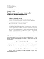
Fig. 1. Comparison of the cross-relaxation rates as a function of 1 H- 1 H distances in a flexible
(
) and rigid protein structure (—). For the flexible protein structure, the ratio of the
cross-relaxation rates between two protons i and j relative to two protons with fixed, known
distances (methylene protons) is estimated as a function Q(Rm) of the maximum distance
between 1 and j , by uniform averaging the interatomic distance between the van der Waals
contact of 2 A and i? m . The estimation was done in such a way that the correct result for Q
should be below the solid line under the assumptions described in the text. Measuring Q
therefore allows a rather conservative estimate of the upper limit of the distance.
(Reproduced from Braun et al. 1981.)

of the maximal distance Rm. The 'maximal' distance is generally defined as the
distance up to which a significant fraction, e.g. 95 % of the population, is occupied:
(2.1.3)

The derivation of equation (2.1.3) is based on two arguments. The first is that

in macromolecular systems the sign of /(T) is negative and the inherent flexibility
of the angular dependence in addition to the overall tumbling can only reduce the
NOE effect:
(2.1.4)

The second argument assumes that the density distribution of the proton-proton
distances behaves well in the sense that the maximum distance Rm and the maximal
value of the density distribution pmax are anticorrelated, i.e. if Rm gets large, /omax
gets small. This assumption is valid for frequently occurring distributions such
as the Maxwellian, Lorentzian or Gaussian distributions, but it excludes cases such
as a two-state model with two delta distributions at a small and a large distance.
The average value <r~8> clearly is not affected much by the maximum distance
for this distance distribution. Such cases might exist in protein structures in

Downloaded from https:/www.cambridge.org/core. University of Basel Library, on 11 Jul 2017 at 10:13:21, subject to the Cambridge Core terms of
use, available at https:/www.cambridge.org/core/terms. />

120

W. Braun

solution. But they seem to be not the statistically dominant cases for proton-proton
distances in proteins; otherwise the proposed direct method would not work at
all. However, by doing distance geometry calculations we sometimes obtain
evidence for averaging processes over at least two conformations (see, for example,
the example of the a-amylase inhibitor in section 4.2).
The ratio (2.1.3) c a n D e estimated as follows:

where rm is the minimal distance available, usually the sum of the van der Waals
radii. When Rm gets large, the right-hand side gets small under our assumption.

This function of Rm on the right-hand side can now be used to estimate for a
measured ratio of the cross-relaxation rates an upper limit for the proton-proton
distance.
A specific model, the uniform averaging model, for calculating Q(Rm) is given
in Fig. 1. This simple model might be replaced by models available from statistical
analysis of molecular dynamic calculations (Olejniczak et al. 1984) or Monte Carlo
simulations. Even if it is not possible to characterize all types of proton—proton
distance distributions in proteins by one general model, certain features of a
statistical analysis of molecular dynamics calculations could be used, e.g. the
observation that distances between proton spins separated by only a few torsion
angles show less variations than long-range distances.
The uniform averaging model has been used in Braun et al. (1983) to determine
the distance constraints for protons separated by at most three torsion angles about
single bonds differently from those for protons separated by more than three
torsion angles. In the first case the rigid model was applied with four classes of
distance limits: 2-4, 27, 3-1 and 4*0 A. In the second case the uniform averaging
model was applied with the same levels of intensities and mixing times but loosened
upper limits. In subsequent protein-structure determinations, a similar scheme
for the translation of NOE cross-peaks into upper limit distance constraints was
used (Williamson et al. 1985; Kline et al. 1986; Braun et al. 1986; Wagner et al.
1987).
The main conclusion is that NMR data in proteins give upper-limit distance
constraints or imprecise distance information with errors comparable to the size
of the distances itself. On the other hand, the number of distance constraints is
much larger than the number of degrees of freedom. The distance constraints
provide us with a large network of restrictions. This fact converts the problem into
a computationally difficult class, which cannot be solved by a fast algorithmus
(Saxe, 1979). This computational problem is comparable-in complexity to the
protein folding problem.

Downloaded from https:/www.cambridge.org/core. University of Basel Library, on 11 Jul 2017 at 10:13:21, subject to the Cambridge Core terms of
use, available at https:/www.cambridge.org/core/terms. />

Protein structure determination from NMR data

121

2.2 Dihedral angles constraints
Vicinal proton-proton coupling is another source of useful geometric information.
The dependence of the vicinal coupling constant between two protons H 1 and H 2
on the dihedral angle <f> is given by a Karplus type equation (Karplus, 1959, 1963):
ã/H'Hô(0)

= -A + B cos0 + Ccos20.

(2.2.1)
3

3

The parameters A, B and C for the vicinal coupling constants J a N H and Ja^ for
polypeptides have been empirically determined by a best-fit procedure for the
measured vicinal coupling constants for systems where also a highly refined X-ray
structure was available. Numerous attempts have been done along these lines to
determine the 'best' set of parameters (cf. De Marco et al. 1978a, b). All of these
calibrations of course assume that the solution structure of a protein used for
calibration is highly rigid and is the same as the X-ray structure. Because of this
basic drawback it is advisable to use geometric information from the measured
coupling constants only when it is insensitive to variations in the parameters used.
In the future, NMR structures of small globular proteins might be used for

calibrating the parameters of the Karplus curve. Pardi et al. (1984) used the X-ray
structure of BPTI (Walter & Huber, 1983) to calibrate the parameters of the
amide proton-C a proton coupling constant 3 J a N H . To get a rough estimate of the
influence on the calibration of taking either structure, differences in the dihedral
angles between the X-ray and a representative NMR structure of BPTI (Wagner
et al. 1987) were calculated. The DISMAN structure 1 of BPTI (see Table 1) was
used as a reference structure for the family of NMR structures. The mean
deviation of the

the X-ray structure for those 46 amino acid residues which have been used in the
calibration study amounts to 240. All residues for which 3 J a N H coupling constants
of 36 or 68 °C were measured have been included in this comparison except the
carboxy terminal Ala-58. This mean deviation corresponds roughly to the scatter
of the experimental data points around the best-fit theoretical curve, fig. 3 in Pardi
et al. (1984).
But even if all the parameters A, B and C were exactly known, flexibility of the
molecule prevents us using equation (2.2.1) in a straightforward way in the direct
determination of polypeptide or protein conformations. The measured values of
the coupling constants are averaged over the ensemble of equilibrium conformations. This fact requires that we use only the extreme values of the vicinal coupling
constants for structural interpretation, because for these extreme values averaging
should not have a major effect. But using only the extreme values of the Karplus
curve of the vicinal coupling constant leads to a rather large inaccuracy in the
dihedral angle obtained from the measured coupling constant.
The fact that averaging processes can only diminish the extreme cases has also
been demonstrated by Nagayama & Wiithrich (1981) in a two-dimensional
representation of the two 3Ja/? coupling constants of the methylene protons whose
dihedral angles are correlated by 1200. They distinguished three limiting cases for
the fluctuations of the x1 angle: the fully rigid case where the experimentally
Downloaded from https:/www.cambridge.org/core. University of Basel Library, on 11 Jul 2017 at 10:13:21, subject to the Cambridge Core terms of
use, available at https:/www.cambridge.org/core/terms. />

122

W. Braun

measured values are at the extreme boundary values, the case of small (300)
fluctuations around a single rotameric conformation where the experimental data
point is near the boundary values, and the case of rapid exchange between at least
two rotamers.
All these considerations on the flexibility of the molecule lead to a similar
conclusion as to which type of dihedral angle constraints can be expected in a
direct-method approach. As in the case of distance constraints, the experiments
define an allowed interval for dihedral angles and the problem consists of finding
all molecular conformers with dihedral angles in these allowed intervals.
3. THEORY

3.1 Formulation of the mathematical problem

Molecular conformations compatible with the NMR data are characterized by
allowed ranges of geometric quantities such as dihedral angles or distances. The
basic question in the determination of protein conformations is to characterize the
conformation space compatible with these constraints. The result of such a
characterization does not consist of a single structure satisfying the experimental
data best but rather of a set of structures where each structure should be considered
as a particular representation of the allowed conformation space. Systematic grid
search calculations through all possible conformations can be done for small
oligopeptides (Smith & Veber, 1986) but is not feasible for protein-structure
determination. Parameters used to characterize the extent of the conformation
space are the average root-mean-square distances (r.m.s. D) between pairs of
structures (McLachlan, 1979) for a subset of atoms or for all atoms, standard
deviations of dihedral angles and stereoviews of superpositions of structures.

The relation between the inaccuracies with which individual geometric quantities are known and the r.m.s. D values which characterize the restriction of the
whole set of restrictions is by no means trivial and is sometimes surprising. A
striking result of this non-trivial relation has been shown by Havel et al. (1979)
in a simplified model of protein conformation. Each residue is represented by its
C a position. For each pair of C a -atoms the contact of two residues is defined if
the C°-C a distance is less than 10 A. Then it was shown that all conformations
having the same contact-noncontact scheme as the globular X-ray conformation
are restricted to about 1 A r.m.s. D value around the X-ray conformation.
The combined effect of qualitative distance information can have a quite
dramatic effect on possible structures. This relation was further analysed by Wako
& Scheraga (1981) in a statistical analysis of these calculations.
Distance information of this type is generally not available from present NMR
techniques and it is unlikely to obtain in the future especially good information
on long distances of the order of the radius of gyration. Even so, these results gave
some hope that the inclusion of the packing restriction in an all-atom model
together with a fine net of short proton-proton distance constraints is enough to
define the globular fold of the protein. The tools to tackle this question were
developed from a variety of different approaches and are described in the following
sections. Having these tools and a good set of distance constraints, it actually could
Downloaded from https:/www.cambridge.org/core. University of Basel Library, on 11 Jul 2017 at 10:13:21, subject to the Cambridge Core terms of
use, available at https:/www.cambridge.org/core/terms. />

Protein structure determination from NMR data

123

be shown that the hope was justified. A clear test for this hypothesis was presented
in the structural determination of the X-ray single crystal and the NMR structure
of a-amylase inhibitor where for the first time an independent structural analysis
of an unknown structure of a globular protein by both methods was done (Pfiugrath

et al. 1986; Kline et al. 1986).
3.2 Metric matrix methods
In the case in which all distances between all pairs of atoms are known exactly,
distances can be converted into cartesian coordinates by an elegant use (Crippen
& Havel, 1978; Crippen, 1981) of the matrix
G

ij

= Tirj>

.

(3-2-0

where rf denotes the cartesian coordinates of atom i and • the dot product. Thus
Gy is a N x JV matrix. The matrix elements of the metric matrix determine the
coordinates uniquely except for a rotation and inversion. The relation is simply
given by diagonalization of the matrix:
N

Gij = I.\aEi,aEj
(3.2.2)

a

This relation can be seen by proving the two important properties of the metric
matrix. The metric matrix is positive semidefinite and has rank 3. This means that
all eigenvalues of the metric matrix are greater than or equal to zero and at most

three eigenvalues are different from zero. This can be derived from the quadratic
form of the metric matrix:
N

tS

\ (N

If the quadratic form is zero one obtains a 3-dimensional vector equation or three
linear equations in the N variables zf:
N

'£ziri = o.

(3-2.4)

i

Therefore there are at least N— 3 linear independent non-trivial solutions, which
means that the metric matrix has at most only three eigenvalues different from zero.
In the general eigenvector decomposition equation (3.2.2) of a metric matrix
corresponding to a set of 3-dimensional coordinates all but three terms vanish
and a comparison of (3.2.1) and (3.2.2) leads to
(3-2.5)
The metric matrix can be calculated directly from the distances. This makes this
quantity important for practical use:

^

^

f

c

,

(3-2.6)
(3-2-7)

Downloaded from https:/www.cambridge.org/core. University of Basel Library, on 11 Jul 2017 at 10:13:21, subject to the Cambridge Core terms of
use, available at https:/www.cambridge.org/core/terms. />

124

W. Braun

In the first of these equations for the diagonal term it is implicitly assumed that
the structure is centred to the origin. Another choice would be setting one
particular atom usually numbered o at the origin:
Gu = r{-ri = DStt.

(3.2.8)

The set of equations (3.2.i)-{3.2.8) gives a simple and direct relation between
distances and coordinates. A detailed mathematical description of these equations
can be found in Havel et al. (1983). The equations are derived on the assumption
that all distances are known exactly, i.e. in the case of a complete and correct
distance matrix. In practical applications these basic assumptions are almost never
fulfilled in typical NMR data sets, but there is a hope that the assumptions still

represent a useful approximation (Braun et al. 1981; Crippen et al. 1981).
As we have seen in the previous section, distance information is given in the form
of an interval,
Ltj^Di}^Uip

(3.2.9)

and usually only for a small subset of all possible atom pairs. In the case of the
a-amylase inhibitor (Kline et al. 1986) there are about 500 distance constraints
from NMR data. These constraints are to be complemented with about 1500
constraints for bond lengths and bond-angle constraints. But this is a small number
compared to all possible atom pair distances, which must be known for all 827
atoms in the pseudo-atom representation (Wiithrich et al. 1983) to generate a full
metric matrix.
Initial distances are chosen at random between the limits given in (3.2.9). This
usually leads to a distance matrix not embeddable in three 3 dimensions, i.e.
the metric matrix calculated from the distances is not positive semidefinite with
rank 3. This means there are no coordinates in 3 dimensions with the same
distances as the randomly chosen distances. In practice the approximation using
the three greatest eigenvalues in equation (3.2.5) to calculate the coordinates is
usually done.
In our experience, with a large system of say N ^ 50 (i.e. even a short
polypeptide chain with all atoms included would be large in this sense) the three
eigenvalues with greatest absolute value are not always positive. This is partially
related to the fact that the randomly chosen distances within bounds satisfying
triangle inequalities do not necessarily satisfy the triangle inequalities among
themselves. This is especially true if the bounds are loose. As a simple example,
let us assume that the upper and lower bounds for the 3 distances of a triangle
are 10 and 2 A, respectively. Then the direct and the inverse triangle inequality
for the upper and lower bounds are satisfied. However, choosing the three

distances at random independently within the allowed range might lead to three
distances not consistent with the triangle inequality (e.g. 10, 2 and 2 A).
Crippen et al. (1981) calculated correlation coefficients between the three
distances of a triangle imposed by the upper and lower bounds. These were then
used in correlating random choices of the initial distances. The probability of
violating the triangle inequality is thereby reduced but not to zero. A different
Downloaded from https:/www.cambridge.org/core. University of Basel Library, on 11 Jul 2017 at 10:13:21, subject to the Cambridge Core terms of
use, available at https:/www.cambridge.org/core/terms. />

Protein structure determination from NMR data

125

solution to correct the triangle inequalities exactly for the distances within the
given bounds was proposed by Braun et al. (1981). In this approach specific
changes for those distances violating the triangle inequality were derived, such that
the new distances are still within the allowed range and satisfy the triangle
inequality. Higher-order inequalities (Havel et al. 1983) restricting further upper
and lower bounds have also been derived but it is not clear if they are of practical
use because of the enormous amount of computing time.
The connexion between diagonalization and coordinates has also been recognized and used in an abstract way by regarding ri as a 3N dimensional vector of
a conformation i and calculating (3.2.1) for a set of M conformations. In this case
G i s a M x M matrix. Two-dimensional projected coordinates of each conformation 1 were then used in a two-dimensional graphical representation of the set of
conformations in the refinement studies of X-ray protein structure determination
(Diamond, 1974) and analysis of molecular-dynamics calculations (Levitt, 1983).
For use in the tertiary structure determination of a polypeptide chain it is not
sufficient to have an embed algorithm; one also has to combine the standard
geometry of individual amino acids (e.g. ECEPP geometric parameters) in a library
with the embed procedure to extract the distance constraints which define the
stereo chemistry.

This was first done in the calculation of micelle-bound glucagon (Braun et al.
1981). A new FORTRAN computer program, based on the metric matrix approach of
Crippen & Havel (1978), was written to model the individual amino acids by
distances. By relying on pure geometrical principles and on simplified representations of protein structures, the distance geometry algorithm (Crippen, 1977,
1981) was designed to circumvent the local minimum problem of empirical energy
minimization (Nemethy & Scheraga, 1977). We intended, however, to use it as
some sort of model building algorithm for polypeptide chains, where the experimental distance information could easily be included as an additional constraint.
In designing the program we had to define the standard bond lengths and bond
angles by distances. This was done by interfacing the metric matrix approach with
the standard amino acid library of ECEPP (Momany et al. 1975). The only
necessary input information for the chemical structure consisted then of the amino
acid sequence. All relevant distance information was automatically read from the
ECEPP library.
The basic EMBED algorithm was extended by using new triangle inequalities
for the distances (see above) to get an improved set of initial distances in the initial
embedding. Truncation of the metric matrix to the space spanned by the
eigenvectors with the three greatest eigenvalues was replaced by a gradual
contraction using a convex combination of old and new distances derived from the
approximate coordinates. This procedure led to an improved set of initial
coordinates for the refinement.
Test calculations also showed that individual chirality terms must be added to
the error function in the refinement procedure to get the correct chirality of the
asymmetric C a carbon atoms of the amino acid residues and the chirality of the
C^ atom of Thr and He. This requirement extended the original scheme of the

Downloaded from https:/www.cambridge.org/core. University of Basel Library, on 11 Jul 2017 at 10:13:21, subject to the Cambridge Core terms of
use, available at https:/www.cambridge.org/core/terms. />

126

W. Braun

metric matrix approach from a pure distance geometry problem towards a
refinement problem.
An extension of the approach along these lines was done in the program DISGEO
(Havel & Wiithrich, 1984), where several new features were included to make this
approach workable also for small proteins in the pseudo-atom representation.
Embedding is done in two steps, where first the conformation of a substructure
consisting only of a subset of a third of the atoms in the complete structure is
calculated and then the distances extracted from the calculated substructures are
relaxed somewhat and included as additional constraints for the embedding of the
complete structure. Even in the pseudo-atom representation, the N2 memory
demand for a small protein is a major problem in this approach. This was solved
by an efficient storage of incomplete distance information and use of disk storage
in cases which are not time-critical. Because of sequential disk access, the
computation of triangle inequality limits on all distances from the given set of input
distance bounds is a highly non-trivial problem and has been solved by
implementing a special shortest-path algorithm. In addition to the chirality
constraints to fix the chirality of the L amino acids, further chirality constraints
were included to force planarity of the peptide planes and the aromatic rings.
Chirality constraints were also used to restrict torsion angles around a single bond
where the ambiguity of the relation between chirality and torsion angles (one
chirality value typically corresponds to two torsion angles) is resolved by using
several dihedral angles around the same chemical bond (Havel & Wuthrich, 1985).
3.3 Future developments
The basic EMBED algorithm proposed first by Crippen & Havel (1978) does not
include any term dealing with the chirality constraints. In our first approach to
use this method to model the individual amino acid residues by distance information, L and D amino acids could not be distinguished by distance information
because a point inversion of a 3-dimensional structure converts a L into a D
configuration leaving the distances invariant. Therefore an ad hoc procedure was

proposed (Braun et al. 1981; Crippen et al. 1981) to include the chirality
constraints in the refinement procedure where a target function of the type
discussed in the next section is minimized. Even though this approach worked in
practice to some extent, it left some burden to the final refinement procedure. An
algebraic embed procedure including chirality constraints still needs to be
developed.
The basic metric matrix approach has two drawbacks if the system is a typical
small protein of the size which can now be studied by 2-D NMR experiments.
For this size the truncation to the three largest eigenvalues of the metric matrix
represents a poor approximation. The memory demand is quadratical in N, the
number of atoms. Even on a virtual memory system this represents a potential
limitation because of paging. It seems that the redundancy of the distance
information has not yet been exploited fully to generate a complete, but small
subset of distances with a size linear in N carrying the necessary 3-dimensional
information.
Downloaded from https:/www.cambridge.org/core. University of Basel Library, on 11 Jul 2017 at 10:13:21, subject to the Cambridge Core terms of
use, available at https:/www.cambridge.org/core/terms. />

Protein structure determination from NMR data

127

Current research (Sippl & Scheraga, 1985, 1986; Schlitter, 1986) is concerned
with the correction or prediction of the undefined distances such that the complete
distance matrix is embeddable. Theorems on necessary and sufficient conditions
on the embeddability (Blumenthal, 1970) are not of much help because in typical
cases the conditions are violated, and the way to satisfy these conditions is then
done by a nonlinear best-fit procedure, i.e. that feature one wanted to avoid at the
outset of this approach. The proposed approach used Caley-Menger coordinates
to fill out a complete distance matrix from a sparse, incompletely defined distance

matrix. This was done by a suitable simplification of the Caley-Menger determinants such that they can be calculated with minimal effort. However, it has
not been demonstrated that this procedure can be used in practice for a molecule
of the size of a protein.
3.4 Variable target function method
As we have seen in the previous section, the mathematical problem of the general
embedding problem is not yet solved. There are mathematical indications that
there might not be a reasonable algorithm to solve it in a reasonable computer time
for large system, because it was shown that this problem is NP hard, i.e. the
number of operations needed to solve that general problem is for any algorithm
not bounded by a polynomial in N (Saxe, 1979).
Practical experience gained with the NMR data of glucagon (Braun et al. 1981,
1983) and preliminary data on the NMR data of BPTI using a simplified two-point
representation for each residue, where one point represents the C a atom and the
other point the side-chain of the residue, suggested that, for larger systems, one
certainly cannot avoid the use of nonlinear optimization at some phase of the
algorithm. Then it is a natural idea to try the nonlinear optimization method from
the outset in a straightforward way.
In the general frame of a nonlinear optimization scheme one should try to keep
the number of independent variables as small as possible (Fletcher, 1980). An
obvious choice are then the torsion angles as independent variables. The problem
of local minima (Nemethy & Scheraga, 1977; Go & Scheraga, 1978) seems
sometimes easier to be solved by artificially enlarging the number of degrees of
freedom (Crippen, 1977; Purisima & Scheraga, 1986), but reduction of the higher
dimensional structures to the 3-dimensional space usually poses additional
problems. So it is not yet clear if the local minima problem is solved by the
above-mentioned procedures or only translated to a different problem. A real
solution of the local minima problem in protein-structure calculations is not just
an ad hoc algorithm proposed to avoid the local minima, but also a realistic picture
of the nature of local minima. This is still missing.
To have a program at hand to treat proteins of the size that can be studied bythe present NMR techniques, a new algorithm was implemented into a FORTRAN

computer program DISMAN (Braun & Go, 1985). This program tries to make best
use of the available data. Knowledge of stereo chemical data such as standard bond
lengths, bond angles and the repulsive core radii have to be added to the pure
experimental data from NMR to start structural elucidation. This is done by
Downloaded from https:/www.cambridge.org/core. University of Basel Library, on 11 Jul 2017 at 10:13:21, subject to the Cambridge Core terms of
use, available at https:/www.cambridge.org/core/terms. />

128

W. Braun

generating the atomic coordinates from the dihedral angles and changing the
dihedral angles in such a way that a target function becomes zero for a structure
which fulfils all distance constraints. The target function is a measure of how good
the distance constraints are fulfilled. There are many ways to construct such target
functions. A typical form of the target function is given by

T= 2
The function 6(x), which is o for x < o and i for x > o, is used to sum up all
distance violations. The summation over the atompairs i and j is, of course, only
over those pairs where there are constraints. The function T is o for a solution,
is positive for all conformations not satisfying the constraints perfectly and
increases as the distance constraints violations are getting worse. Usually the target
functions are variations of the type (3.4.1) that only the square of distances is used
because of efficient computation and such that they are also continuously
differentiable at the boundaries D(j = L y and Z>y = Uy. This can be done by taking
some powers of the distance violations (see, for example, Braun et al. 1981).
Summing up only terms which represent distance violations can be done without
any discontinuity of the derivative. This approach yields a clear correspondence
between a solution and T = o, which is a definite advantage of distance geometry

calculations over energy minimization where such a priori knowledge of the global
minimum is missing. This advantage is lost if one uses the approach of Marion
et al. (1986) of including terms when the distance constraints are satisfied.
The variable target function approach is not entirely new, because computation
in torsion angle space has been done extensively in energy minimization studies
of proteins (Burgess & Scheraga, 1975; Meirovitch & Scheraga, 1981; Levitt,
1982, 1983). Two new features are an efficient way to calculate gradient information
of the target function (Noguti & Go, 1983; Abe et al. 1984) and the way the target
function in (3.4.1) is minimized. Our strategy of minimizing is similar to the
strategy of Ooi et al. (1978) in the regularization studies of proteins.
The method of variable target functions means that one does not try to minimize
T at once but rather to minimize gradually a series of functions which approximate
T. More specifically, for a polypeptide chain of n residues the target functions Tk l
(As = 1, 2, . . . , n and / = 1, 2, . . . , n) only include those terms of the form as in
(3.4.1) for atom pairs belonging to residues with difference of their sequence
numbers less than k if the upper or lower limits are from NMR data or less than
/ if the lower limits are the sum of repulsive core radii. The strategy consists in
first minimizing Tk t with small values of k and / and then gradually increasing
k and / up to n. The final solution of the problem consists of one or several
conformations having zero values for Tn n= T. The exact definition of the terms
used in DISMAN can be found in (Braun & Go, 1985). In case of an overdetermined
problem the best conformation consistent with the input distance information and
stereo-chemical criteria is the one which gives the global minimum of the target
function.
This strategy was shown to be effective if good distance information of a short
range nature is available. In the case of artificial distance data with exact
Downloaded from https:/www.cambridge.org/core. University of Basel Library, on 11 Jul 2017 at 10:13:21, subject to the Cambridge Core terms of
use, available at https:/www.cambridge.org/core/terms. />

Protein structure determination from NMR data

129

proton-proton distances less than 5 A, the polypeptide backbone structure of
BPTI could be almost exactly regenerated with r.m.s. D values of 003 to 014 A.
The calculations started with ten randomly chosen initial conformations differing
from each other and from the final structures by about 15 A (Braun & Go, 1985).
In practice this good distance information is certainly not available; however, good
distance information of a short-range nature is always obtained in the process of
sequential resonance assignments (Wagner & Wiithrich, 1982 a) and measurements
of spin—spin coupling constants can be used directly to restrict the allowed torsion
angles.
Exact characterization of good distance information which can guide the
conformation from correct short-range to medium or long-range conformations
is missing. More extensive numerical experience is certainly needed. Some
heuristic ideas of describing the success of the method are as follows. Short-and
long-range distance constraints impose different types of restrictions on the
polypeptide conformation. Once short-range distance constraints are fulfilled, the
polypeptide chain keeps a large amount of 'flexibility' for those conformational
changes maintaining the short-range distance information. Small local changes
can give rise to drastic global changes. So these small changes can be used to satisfy
the long-range distance constraints.
In DISMAN certainly, only a specific aspect of the variable target function method
is implemented. In future a cybernetic choice of the target function using feedback
methods could give improved results. Now, information on the success or failure
of a certain run is not used in the calculation of further conformations. Also, a
combination with Monte Carlo Methods of escaping local minima might be a
possibility to improve the performance of the method.
The second device implemented in DISMAN is a method of fast calculation of
the gradient of the target function. A different scheme has been proposed

independently by Levitt (1983). It is therefore of some interest to see the relation
between these schemes. Both methods can be applied either to an empirical energy
function or to the target function of the type (3.4.1). To make the comparison
transparent we describe it in the notation of Abe et al. (1984) for numbering the
atoms and the dihedral angles. Atom indices are denoted by Greek letters a,fi,y,...
and torsion angle indices by a, 6, c, . . . .
The basic idea in the first scheme of efficient calculation of the gradient was
introduced by Noguti & Go (1983). It relies on the 'factorization' of the terms
in the gradient into quantities dependent on torsion angles and quantities
dependent on individual atoms and of the grouping of all atoms in the molecule
into units Va attached to each rotatable bond. Each unit consists of one or more
atoms. Units are defined by the property that there are no rotatable bonds within
them and therefore the relative positions of atoms within each of them remain fixed
for any conformational changes of the molecule. The gradient of a function E,
which is a sum over pairwise distance dependent potentials 0a/J (|ra — r^|) is given
by
dE
•30- = - e o • F a ~ (e B A r £ ( a ) ) G o ,

(3. 4 > 2 )

Downloaded from https:/www.cambridge.org/core. University of Basel Library, on 11 Jul 2017 at 10:13:21, subject to the Cambridge Core terms of
use, available at https:/www.cambridge.org/core/terms. />

130

W. Broun

where F o and G a are calculated via simple recurrent equations:
p(a)

F

a =fo+Ê

F

ô(fc,o)>

(3-4-3)

fc-1
p(a)
G

8 <*.

a) ã

(3-4-4)

(3-4-5)
(3-4-6)
The indices s(k, a) k = i, 2, . . . , p(a) describe the hierarchical tree structure of
a branched polymer. It gives for each rotatable bond a the indices of the torsional
angles branching from bond a and p(a) counts the branches at a. The order of the
torsion angles is chosen appropriately (Abe et al. 1984).
Because of the grouping of the atoms in no-overlapping units, all auxiliary
quantities fa and g 0 can be calculated in N2 number of operations and the result
stored appropriately. The summation of the recurrent equations and the
calculation of the individual components of the gradient (3.4.2) is then done in a

second phase where the calculational effort is on the order of m, the number of
torsional angles.
In the second scheme (Levitt, 1983) first derivatives are calculated with respect
to all cartesian coordinates and stored.

This can be done in N2 number of operations. In a second step these derivatives
are transformed to torsion angle space:
^

= 2|^-[e0A(ra-r6(a))].

(3.4.8)

This second step needs only Nxm number of operations.
Both methods are mathematical equivalent because of the following relation:
(ra-r^-[9aA(ra-r
=-ea-(raAr^)~{eaAre{a))-(ra-rfi).

(3.4.9)

Both methods have roughly the same efficiency and are a factor N faster than
straightforward analytical (Pottle et al. 1980) or numerical methods. The first
method needs less memory space because the recurrent equations can be implemented using a stack method. In practice, however, this is not a crucial advantage.
This is important, however, for the second derivative method. The first method
has been implemented to calculate analytical second-order derivatives in the
normal mode analysis (Go et al. 1983) where other methods use analytical firstand numerical second-order derivatives (Levitt et al. 1985). The first method can
also easily extended to systems consisting of two or more molecules (Braun et al.
Downloaded from https:/www.cambridge.org/core. University of Basel Library, on 11 Jul 2017 at 10:13:21, subject to the Cambridge Core terms of
use, available at https:/www.cambridge.org/core/terms. />

Protein structure determination from NMR data

131

1984), which is important for studying enzyme-substrate systems. In this extension
the rotation and translation parameters (translation vectors and Eulerian angles for
rotation) can be embedded in a natural way in the hierarchical tree structure and
are used formally as torsion angles.
Explicit restrictions on torsional angles from spin-spin coupling constants
(Karplus, 1959; DeMarco et al. 1978 a; b) can be implemented easily. This is done
in DISMAN following the same philosophy used in constructing the target
function from distance constraints. For each restricted torsion angle to an allowed
region, i.e. to a region compatible with the NMR data, the target function is denned
as zero within the allowed region, has continuous first derivatives at both region
boundaries and increases smoothly with the amount of deviation from the allowed
region. Some care has to be taken, because the 3-dimensional coordinates are 2n
periodic functions of the torsion angles. Also the evaluation of the function should
be fast. In DISMAN a fourth-order polynomial with continuous first derivatives and
2TT periodicity is constructed.
If [0L, 0jj denotes the allowed region where all angles have been scaled to
radians, we can always achieve the condition
o^0R-eL^2n.

(3-4-io)

This means in practice that if we want to restrict the angle near 1800, we have to
choose the left and right limits of the angle interval in degrees below and above
1800. The allowed region can also be characterized by its mean value m and width
w where

™ = K0R+0L);

H> = i(0 R -0 L )-

(3.4.")

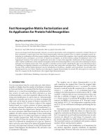
The deviation Ad of the current torsion angle from its mean value is also
27r-periodic and can be always shifted in the interval [o, 2ir\. The allowed region
splits by this shift in two separate regions, [o, w] and [zn — zv, ZTT\; and the
forbidden region therefore remains in one contiguous segment \w, zn—w\. This
transformation of the allowed regions in the variable 6 and in the deviation from
the mean value m, Ad, are schematically sketched in Fig. 2 by the hatched areas.
By transforming the deviation Ad by
~
Ad-it
Ad =
n—zv

,
.
(3-4-12)

the forbidden region is shifted to [— 1, +1] and the target function is defined as

T and its first derivative are continuous also at the boundary A§ = + 1 . The
singular point of the transformation (3.4.12) occurs at w = n, i.e. there is no
restriction on the original torsional angle 0 R = 0 L + 27r. This singular point and a
small neighbourhood can therefore be always avoided. The practical interesting
point of fixing the angle to one particular value by 0 R = dh means w = o and
poses no particular singularity problems.

Downloaded from https:/www.cambridge.org/core. University of Basel Library, on 11 Jul 2017 at 10:13:21, subject to the Cambridge Core terms of
use, available at https:/www.cambridge.org/core/terms. />

132

W. Braun

\—E/

S

/

S

s^.

^~ S

s s
S

S \

I
2JT

V//A

!///;!
w

2ir—w

T

Ke
-1
+1
Fig. 2. Graphical representation of the transformations used in the definition of the target
function for torsion-angle restrictions. The letters m and to denote the midpoint and the
width of the allowed interval for 6 which is drawn as the hatched segment at the top line.
The deviation A0 of the torsion angle from the mean value m is shifted into the interval
[o, 2n] and the allowed area for it is therefore split into the two hatched segments indicated
in the middle line. At the Jsottom the graph of the target function T is schematically
sketched as a function of Ad.
The procedure can also be easily extended to several allowed regions by first
ordering the allowed intervals [0^, #|J (z = i, 2, . . . ) and shifting each forbidden
interval [6^, d^1] by a slightly modified equation (3.4.12) into [—1, +1] and apply
(3.4.13). This implementation is of some practical importance in the stereospecific
resonance assignment.
The variable target function method certainly has some resemblance to restrained energy minimization in torsion angle space (Levitt, 1983). Both methods
use torsion angles as independent variables and are minimizing functions of a
similar type in the torsion angle space. The basic difference is the fact that in the
variable target function method a series of target functions Tk , are minimized
rather than a certain pseudo energy function. This approaches the local minima
problem in a quite different way from modification of the infinite repulsion energy
terms by finite models for overlap atoms ('soft atoms'). This means that in the
stage of the minimization of Tfc , all atom pairs whose residue numbers differ by

more than / can freely penetrate each other, whereas there is still some barrier in
the soft atom model. Also the restraints or constraints are brought differently into
play by the two methods.
However, apart from these more technical differences, the main difference is the
philosophy of the approach. We are mainly concerned with the direct structural
consequences of the pure NMR data with the least amount of additional assumptions. These are stereo chemical data like bond lengths, bond angles and van der
Waals or repulsive core radii. The relevance of a structure found by restrained
energy minimization (this method has not yet been applied to a typical artificial
or experimental NMR data set for proteins) is difficult to judge. Is it mainly
Downloaded from https:/www.cambridge.org/core. University of Basel Library, on 11 Jul 2017 at 10:13:21, subject to the Cambridge Core terms of
use, available at https:/www.cambridge.org/core/terms. />

Protein structure determination from NMR data

133

determined by the energy or by the restraining terms? The fact that empirical
energy calculations have not yet succeeded in predicting the correct global fold
of proteins in solution indicates that the additional energy terms are mainly an
additional burden to the calculation without guiding the minimizer to the correct
global fold. Of course the structures found by the variable target function methods
might have quite unrealistic high energies. So these structures should be further
treated with an energy program which will change the conformation minimally but
will reduce the energy drastically. A suitable tool for this seems to be the
Newton-Raphson minimizer (unpublished results), which can find the next local
minima most efficiently. Escaping the local minimum is in my opinion an undesirable property at that stage. The need to avoid any unnecessary burden in the
calculation comes from the requirement to explore the vast conformation space as
largely as possible. Improving the efficiency of the present algorithms, adapting
them to the next generation of supercomputers and avoiding any computational
load not dictated by the experimental data might then allow them to generate

statistically significant ensembles of structures. The number of solutions found
today in typical application (see Section 4) are of course only case studies.
3.5 Restrained molecular dynamics
Restrained molecular dynamics (MD) has been shown to be an additional valuable
tool in elucidating the molecular conformations compatible with NMR data
(Kaptein et al. 1985; Clore et al. 1985; Bninger et al. 1986). Existing computer
programs for MD calculations (van Gunsteren & Berendsen, 1982; Brooks et al.
1983) have been modified to allow inclusion of the NMR data. This is done by
adding a pseudo pair potential of the form
N0E

~ I W ' , , - ' ? / if '„<'!,•

(3-S

}

to the potential function used in the free dynamics. The target distances r^ are
estimated from the NOE intensity cross-peaks using the r~6 dependence. The force
constants cx and c2 are chosen in such a way that if the deviations of the actual
distances r y from their target distances r^ are equal to the estimated errors of r^
the pseudo energy C/ N O E increases by \kT. These additional harmonic pseudo
forces act like ' strings' between those atom pairs constrained by the NMR data
and drive the molecular conformations towards conformations compatible with
the NMR data. In some calculations (Kaptein et al. 1985) c2 is also set to zero.
In that way only the positive evidence of a NOE cross-peak is taken into account.
The numerical integration schemes used to solve Newton's equations of
motions are described in the papers mentioned above and will not be repeated
here. Our primary interest is: in what respect do these programs use NMR data
and what can one learn from these calculations ?

Restrained MD calculations of protein conformations using NMR data have
been done with two different aims. One aim was the refinement (Kaptein et al.
1985) of a model built structure of the lac repressor head piece (Zuiderweg et al.
Downloaded from https:/www.cambridge.org/core. University of Basel Library, on 11 Jul 2017 at 10:13:21, subject to the Cambridge Core terms of
use, available at https:/www.cambridge.org/core/terms. />

134

W. Broun

1984) that crudely satisfies the NOE distance constraints. The global fold of the
polypeptide chain, in this specific case the relative position and orientation of three
a-helices, is already determined by the model built structure. Restrained MD is
then used to decrease both the potential energy and the pseudo energy C/ N O E
arising from the NOE distance constraints and to study time-dependent effects
(local correlation time and time-averages of geometric quantities related to NOE
data) of the trajectories of the modified dynamics by (3.5.1).
In a more ambitious use of restrained MD (Clore et al. 1985; Brunger et al.
1986) the aim is similar to that in the two previously described methods, to
establish the global fold of the polypeptide chain purely on the basis of the NMR
distance constraints and independently of the initial conformations. Starting
conformations were chosen with either extended or helical segments that
could be assigned by typical NOE pattern (Wiithrich et al. 1984). Initial and final
structures differ by r.m.s. D values of the size of the molecule. Applications of this
method to real experimental NMR data have not yet been reported. In the case
of an artificial distance data set for the protein crambin (Brunger et al. 1986),
folding of the structure by this method was successful with distance constraints
which can be obtained in principle by NMR. The way the distance constraints
were included in the calculations is similar to the strategy used in the variable target
function method. First, the molecular dynamics calculations were done by

including only short-range distance constraints for 2 and 5 ps and by starting from
a completely extended conformation. After 500 cycles of conjugent gradient energy
minimization with the short-range constraints, several phases of restrained
molecular dynamics with all distance constraints and increasing weight factors for
them were done.
3.6 Analysis of structures
The considerations on the internal flexibility of proteins in Section 2.1 and 2.2
explained that the central problem for the NMR structure determinations of
proteins is not a nonlinear best-fit problem of the structure to a number of
measured parameters. It is the characterization of the conformation space of all
structures compatible with all constraints. Several parameters have been used to
quantify this aspect of the structure determination.
First the structures should be consistent with the NMR constraints. In the ideal
case there should be no constraints violations at all. In practice statistics of the
number and size of the residual violations should be presented to judge the quality
of the obtained structures. The sum of distance violations divided by the number
of distance constraints (the average distance violation) would be a quantity in [A]
which could be used to compare the quality of calculations with different data sets
and different proteins. It is roughly the equivalent of the R-factor used in the X-ray
structure determination.
Using only a small subset of the cross-peaks of the NOESY spectra, i.e. a small
subset of distance constraints, it is in general quite easy to generate structures with
small average-distance violation. But then the variations of the calculated
Downloaded from https:/www.cambridge.org/core. University of Basel Library, on 11 Jul 2017 at 10:13:21, subject to the Cambridge Core terms of
use, available at https:/www.cambridge.org/core/terms. />

Protein structure determination from NMR data

135

structures might be large. Quantities measuring the variations of the structures
are root-mean-square distances (r.m.s. D) between pairs of structures for a subset
of atoms or for all atoms (see McLachlan, 1979, for definition, history of use and
a fast way of calculating r.m.s. D values). Depending on the subset of the atoms
used in the calculation for the r.m.s. D, the value is a measure of local or global
conformational variations. Important quantities are the r.m.s. D values for the
backbone structure (BB) or the restricted side-chain representation (Braun et al.
1983). Variations of the local conformations comparing two conformations can also
be quantified by averages of the differences of torsion angles over all residues for
the torsion angles <j>, \jr or x1, DHAD values (Havel & Wuthrich, 1985). The extent
of the conformation space of all structures is measured by using the average values
over all pairs of conformations. More sophisticated parameters such as the
' volume' of the allowed conformation space are difficult to estimate from the few
calculated structures.
Additional methods to visualize the variations are stereo views of optimal
superposed structures. They usually show quite clearly those parts of the NMR
structures least constrained by the data.
A further method to judge the quality of NMR structures is the calculation of
NOESY spectra from the ensemble of calculated structures. Comparing them with
the experimental NOESY spectra represents an objective test of the extent
of the used distance constraints. In the case of the experimental data sets of
metallothionein (see Section 4.2.7), preliminary methods were encouraging
(unpublished results).
4. APPLICATIONS

Applications of the programs to calculate structures compatible with distance
constraints have been done with two different types of distance constraints data
sets.
With the first type, the distance constraints were extracted from known X-ray
structures. In the calculations with these simulated distance constraints sets (Havel

& Wuthrich, 1985; Braun & Go, 1985; Briinger et al. 1986) one first wants to
demonstrate that, for a sufficient complete distance constraints data set, the
calculated structures converge to the structure from which the distances were
extracted. Also one wants to explore the theoretical structural consequences of
distance data sets to set guidelines for the experimental work. What structural
features can be expected in a typical experimental data set ? Which additional data
can significantly improve the structures? Present calculations already indicate
where improvements of the structures can be expected.
A systematic exploration and a theoretical analysis of the correlation between
distance constraints data sets and their structural restrictions is still missing but
the described computational tools in Section 3 above, together with the availability
of supercomputers, can give us in the next few years the necessary data base to
understand in more detail the restrictions imposed by short proton—proton
distances on the protein conformations. This question, besides of being important

Downloaded from https:/www.cambridge.org/core. University of Basel Library, on 11 Jul 2017 at 10:13:21, subject to the Cambridge Core terms of
use, available at https:/www.cambridge.org/core/terms. />

136

W. Broun

in the structure determination in solution by NMR data, also has some relevance
for the prediction of the tertiary structure of proteins by empirical energy
calculations (Nemethy & Scheraga, 1977), because the main part of the nonbonded interactions is of short-distance range compared to the radius of gyration
of a typical globular protein.
The second type consists of the real experimental NMR data sets. In these
distance constraints data sets it is not a priori clear that a solution exists at all; and
if there is a solution whether it is a unique solution. Calculations of protein
conformations compatible with the NMR data, besides giving an objective and

quantitive measure of the restriction of the NMR data, are also an independent
check of the sequence-specific resonance assignment (Dubs et al. 1979; Wagner
& Wuthrich 1982a).
4.1 Simulated data sets
Calculations of protein conformations with simulated data sets have so far been
reported for bovine pancreatic trypsin inhibitor BPTI (Havel & Wuthrich, 1984;
1985; Braun & Go, 1985) and crambin (Briinger et al. 1986). The number of
calculated structures per given data set in all of these studies were rather limited
(typically three structures), so the reported r.m.s. D values have to be taken with
some care.
The three methods reported here use very different approaches to fold a protein
under the influence of the distance constraints. In all three cases the distance
constraints data sets were chosen from those short-distance constraints that can
be expected to be determined by NMR methods (i.e. shorter than 4 or 5 A). The
results obtained clearly demonstrate that the global features of a structure
calculated from present NMR data sets are reliable, despite the fact that all
experimentally accessible distances are short compared to the diameter of the
molecules. This observation contradicts popular criticism (see, for example,
Schmidt & Kuntz, 1984). However, this does not mean that every experimental
distance constraints data set leads to uniquely defined global structure. In each
application of one of the described methods it is necessary to show the structural
restriction of the data.
As an illustrative example of the type of calculations, the results of the DISMAN
calculations with several distance constraints data sets of BPTI are presented
(Braun & Go, 1985). In test calculations of this type one has to separate the
influence of the starting conformations from the influence of the data set. The
approach taken in this study was therefore first to generate ten structures by
choosing the variable dihedral angles randomly. The r.m.s. D values comparing
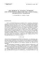
all pairs of initial structures ranged from around 8 to 22 A. A typical example of
one of these initial structures is shown in Fig. 3. This set of initial structures was

then used as starting conformation with several data sets. By using the most
stringent data set (EX5), where all exact short proton-proton distances less than
5 A have been used as constraints, the polypeptide backbone of BPTI was nearly
exactly regenerated with r.m.s. D values ranging from o-oi to 015 A by starting
Downloaded from https:/www.cambridge.org/core. University of Basel Library, on 11 Jul 2017 at 10:13:21, subject to the Cambridge Core terms of
use, available at https:/www.cambridge.org/core/terms. />

Protein structure determination from NMR data

137

Fig. 3. Stereo view of one of the ten initial random structures of BPTI used in the
calculations of DISMAN with the simulated data sets. For clarity only the heavy atoms are
shown. In the calculations all hydrogen atoms are included.

from the ten randomly chosen initial structures. This again shows that short
proton—proton distances are potentially a quite powerful source of information for
restricting the global polypeptide fold.
Data sets of the type experimentally available by the present NMR techniques
are the data sets AL5 and AU5 defined below. Both data sets consists of shortand long-range constraints. Short-range distance constraints were defined as
constraints between the protons NH, H a and H^, which belong to residues
separated sequentially by 2 or less intervening residues. Intraresidue constraints
were deliberately excluded, because the stereospecific assignment of the methylene
protons (a tedious and difficult procedure) for all residues is required. These
distance types were put into six classes from 2 to 5 A with an interval of 0-5 A.
The upper and lower bound distance constraints were defined as the upper and
lower bounds of the class to which it belongs. In AU5 only the upper bounds for
the short-range constraints were used, in AL5 upper and lower bounds were
included. For the long-range constraints upper limit distance constraints were set
in both data sets to 5 A if the corresponding proton-proton distance were less than

5 A. So the two data sets differ in the short-range data sets where in AL5 also lower
limits have been included. Since quantification of lower limits from the NOE data
is difficult because of the inherent flexibility of the protein, we want to study the
theoretical implications for the structure by this data set.
Both data sets were used in calculations with the same initial random structures.
Because of restricted computer time we had to choose three among the ten
previously generated initial conformations. The average r.m.s. D values comparing
the calculated structures with the BPTI X-ray structure for the data set AL5 were
1 "4 and 23 A for backbone and all atoms, respectively, and 1-5 and 25 A for AU5.
The result indicates that the differences in the restrictions of structures between
the data sets AL5 and AU5 is not significant. In Fig 4 the heavy atom representation
of calculated structures with AL5 (A) and AU5 (B) superposed to the BPTI X-ray

Downloaded from https:/www.cambridge.org/core. University of Basel Library, on 11 Jul 2017 at 10:13:21, subject to the Cambridge Core terms of
use, available at https:/www.cambridge.org/core/terms. />

B

Fig. 4. Stereo view of the heavy atom structures calculated by DISMAN with the distance
constraints data set AL5 (Fig. 4A) and AU5 (Fig. 4B). In both cases all heavy atoms of the
calculated structures were best fit to the heavy atom of the X-ray structure of BPTI. Starting
conformation for both structures is the structure shown in Fig. 3.

structure is shown. Both structures were calculated starting from the initial
conformation of Fig. 3. Also in this figure, the coincidence of the calculated
structures with the BPTI X-ray structure is similar for both data sets. Remarkably
well defined are the side-chain conformations of the interior side-chain, especially
the orientation of the aromatic ring planes, even though the long-range distance
constraints were chosen in both data sets with a rather loose upper bound of 5 A.
This indicates that part of this restriction is certainly due to the packing constraints

in the interior of the globular protein (Richards, 1974).
For simulated data sets, the three methods have not yet been tested with exactly
the same data sets. So it is too early to judge the sampling property of each method.
Downloaded from https:/www.cambridge.org/core. University of Basel Library, on 11 Jul 2017 at 10:13:21, subject to the Cambridge Core terms of
use, available at https:/www.cambridge.org/core/terms. />

Protein structure'determination from NMR data

139

In the calculation with the experimental BPTI data, care was taken that the two
programs DISGEO and DISMAN used exactly the same data sets. So the results
obtained from that study give indications on the sampling property of the two
programs.
4.2 Experimental data sets
Only work dealing with calculation of protein structures from experimental NMR
data sets is included in the following list. Papers dealing with small polypeptide
chains have been included as well if the work can be considered as an immediate
precursor in the development of methods for the structure determination of
proteins.
4.2.1 Micelle-bound glucagon
This study (Braun et al. 1981, 1983) of the polypeptide hormone glucagon bound
to perdeuterated dodecylphosphocholine micelles (MB-glucagon) was the first
systematic application of the combined use of distance geometry calculations and
NOE data to determine the secondary and tertiary structure of a polypeptide. The
uniform averaging model (see Section 2.1) proposed in this work was an attempt
to include effects of the internal flexibility of the molecule. The partial success of
a detailed atomic structure determination of this molecule from a set of semiquantitative NOE measurements and the existence of a computer program to
generate structures from the experimental NOE data stimulated improvements in
recording NOESY spectra and motivated the collection of rather large distance

constraints data sets of proteins (Arseniev et al. 1984; Zuiderweg et al. 1984;
Williamson et al. 1985; Braun et al. 1986; Kline et al. 1986; Wagner et al. 1986).
In the second paper (Braun et al. 1983) a more detailed study containing a larger
input constraint data set was used to calculate structures. Also a first step was taken
towards a more realistic estimate of the upper-limit distance constraints by a
combination of a rigid and flexible model. Calculations were done for 4 overlapping
segments of 11 residues because NOE data in this system were only available
between those residues which differ in their residue number by at most 4 residues
and the memory restrictions of the metric matrix approach limited us to about that
size of polypeptides.
In this paper we also introduced several parameters to evaluate the quality of
the obtained structures. The variations of the structures were quantified by the
r.m.s. D values of different atom representations. Important are the r.m.s. D values
for the backbone structure (BB) and the restricted side-chain representation (SR)
where only atoms of complete side-chains were included in the best-fit
superposition for those residues with NOEs involving the peripheral hydrogen
atoms. Both values for the four segments showed a good negative correlation with
the number of distance constraints within the segments. Smaller r.m.s. D values
prevail for those segments with a larger set distance constraints. The backbone
r.m.s. D values for the best-defined segments were of the order of 1 A, thus

Downloaded from https:/www.cambridge.org/core. University of Basel Library, on 11 Jul 2017 at 10:13:21, subject to the Cambridge Core terms of
use, available at https:/www.cambridge.org/core/terms. />