AN INTRODUCTION TO MATHEMATICAL OPTIMAL CONTROL THEORY VERSION 0.1 pptx
Bạn đang xem bản rút gọn của tài liệu. Xem và tải ngay bản đầy đủ của tài liệu tại đây (999.93 KB, 125 trang )
AN INTRODUCTION TO MATHEMATICAL
OPTIMAL CONTROL THEORY
VERSION 0.1
By
Lawrence C. Evans
Department of Mathematics
University of California, Berkeley
Chapter 1: Introduction
Chapter 2: Controllability, bang-bang principle
Chapter 3: Linear time-optimal control
Chapter 4: The Pontryagin Maximum Principle
Chapter 5: Dynamic programming
Chapter 6: Game theory
Chapter 7: Introduction to stochastic control theory
Appendix: Proofs of the Pontryagin Maximum Principle
Exercises
References
1
PREFACE
These notes build upon a course I taught at the University of Maryland during the fall
of 1983. My great thanks go to Martino Bardi, who took careful notes, saved them all
these years and recently mailed them to me. Faye Yeager typed up his notes into a first
draft of these lectures as they now appear.
I have radically modified much of the notation (to be consistent with my other writ-
ings), updated the references, added several new examples, and provided a proof of the
Pontryagin Maximum Principle. As this is a course for undergraduates, I have dispensed
in certain proofs with various measurability and continuity issues, and as compensation
have added various critiques as to the lack of total rigor.
Scott Armstrong read over the notes and suggested many improvements: thanks.
This current version of the notes is not yet complete, but meets I think the usual high
standards for material posted on the internet. Please email me at
with any corrections or comments.
2
CHAPTER 1: INTRODUCTION
1.1. The basic problem
1.2. Some examples
1.3. A geometric solution
1.4. Overview
1.1 THE BASIC PROBLEM.
DYNAMICS. We open our discussion by considering an ordinary differential equation
(ODE) having the form
(1.1)
˙
x(t)=f(x(t)) (t>0)
x(0) = x
0
.
We are here given the initial point x
0
∈ R
n
and the function f : R
n
→ R
n
. The unknown
is the curve x :[0, ∞) → R
n
, which we interpret as the dynamical evolution of the state
of some “system”.
CONTROLLED DYNAMICS. We generalize a bit and suppose now that f depends
also upon some “control” parameters belonging to a set A ⊂ R
m
; so that f : R
n
×A → R
n
.
Then if we select some value a ∈ A and consider the corresponding dynamics:
˙
x(t)=f(x(t),a)(t>0)
x(0) = x
0
,
we obtain the evolution of our system when the parameter is constantly set to the value a.
The next possibility is that we change the value of the parameter as the system evolves.
For instance, suppose we define the function α :[0, ∞) → A this way:
α(t)=
a
1
0 ≤ t ≤ t
1
a
2
t
1
<t≤ t
2
a
3
t
2
<t≤ t
3
etc.
for times 0 <t
1
<t
2
<t
3
and parameter values a
1
,a
2
,a
3
, ···∈A; and we then solve
the dynamical equation
(1.2)
˙
x(t)=f(x(t), α(t)) (t>0)
x(0) = x
0
.
The picture illustrates the resulting evolution. The point is that the system may behave
quite differently as we change the control parameters.
More generally, we call a function α :[0, ∞) → A a control. Corresponding to each
control, we consider the ODE
(ODE)
˙
x(t)=f(x(t), α(t)) (t>0)
x(0) = x
0
,
3
x
0
α = a
1
t
1
t
2
t
3
trajectory of ODE
time
α = a
3
α = a
2
α = a
4
Controlled dynamics
and regard the trajectory x(·) as the corresponding response of the system.
NOTATION. (i) We will write
f(x, a)=
f
1
(x, a)
.
.
.
f
n
(x, a)
to display the components of f, and similarly put
x(t)=
x
1
(t)
.
.
.
x
n
(t)
.
We will therefore write vectors as columns in these notes and use boldface for vector-valued
functions, the components of which have superscripts.
(ii) We also introduce
A = {α :[0, ∞) → A | α(·) measurable}
to denote the collection of all admissible controls, where
α(t)=
α
1
(t)
.
.
.
α
m
(t)
.
4
Note very carefully that our solution x(·) of (ODE) depends upon α(·) and the initial
condition. Consequently our notation would be more precise, but more complicated, if we
were to write
x(·)=x(·, α(·),x
0
),
displaying the dependence of the response x(·) upon the control and the initial value.
PAYOFFS. Our overall task will be to determine what is the “best” control for our
system. For this we need to specify a specific payoff (or reward) criterion. Let us define
the payoff functional
(P) P [α(·)] :=
T
0
r(x(t), α(t)) dt + g(x(T )),
where x(·) solves (ODE) for the control α(·). Here r : R
n
× A → R and g : R
n
→ R are
given, ane we call r the running payoff and g the terminal payoff. The terminal time T>0
is given as well.
THE BASIC PROBLEM. Our aim is to find a control α
∗
(·), which maximizes the
payoff. In other words, we want
P [α
∗
(·)] ≥ P[α(·)]
for all controls α(·) ∈A. Such a control α
∗
(·) is called optimal.
This task presents us with these mathematical issues:
(i) Does an optimal control exist?
(ii) How can we characterize an optimal control mathematically?
(iii) How can we construct an optimal control?
These turn out to be sometimes subtle problems, as the following collection of examples
illustrates.
1.2 EXAMPLES
EXAMPLE 1: CONTROL OF PRODUCTION AND CONSUMPTION.
Suppose we own, say, a factory whose output we can control. Let us begin to construct
a mathematical model by setting
x(t) = amount of output produced at time t ≥ 0.
We suppose that we consume some fraction of our output at each time, and likewise can
reinvest the remaining fraction. Let us denote
α(t) = fraction of output reinvested at time t ≥ 0.
5
This will be our control, and is subject to the obvious constraint that
0 ≤ α(t) ≤ 1 for each time t ≥ 0.
Given such a control, the corresponding dynamics are provided by the ODE
˙x(t)=kα(t)x(t)
x(0) = x
0
.
the constant k>0 modelling the growth rate of our reinvestment. Let us take as a payoff
functional
P [α(·)] =
T
0
(1 −α(t))x(t) dt.
The meaning is that we want to maximize our total consumption of the output, our
consumption at a given time t being (1 − α(t))x(t). This model fits into our general
framework for n = m = 1, once we put
A =[0, 1],f(x, a)=kax, r(x, a)=(1− a)x, g ≡ 0.
0
T
t*
α* = 1
α* = 0
A bang-bang control
As we will see later in §4.4.2, an optimal control α
∗
(·) is given by
α
∗
(t)=
1if0≤ t ≤ t
∗
0ift
∗
<t≤ T
for an appropriate switching time 0 ≤ t
∗
≤ T . In other words, we should reinvest all
the output (and therefore consume nothing) up until time t
∗
, and afterwards, we should
consume everything (and therefore reinvest nothing). The switchover time t
∗
will have to
be determined. We call α
∗
(·)abang–bang control.
EXAMPLE 2: REPRODUCTIVE STATEGIES IN SOCIAL INSECTS
6
The next example is from Chapter 2 of the book Caste and Ecology in Social Insects,
by G. Oster and E. O. Wilson [O-W]. We attempt to model how social insects, say a
population of bees, determine the makeup of their society.
Let us write T for the length of the season, and introduce the variables
w(t) = number of workers at time t
q(t) = number of queens
α(t) = fraction of colony effort devoted to increasing work force
The control α is constrained by our requiring that
0 ≤ α(t) ≤ 1.
We continue to model by introducing dynamics for the numbers of workers and the
number of queens. The worker population evolves according to
˙w(t)=−µw(t)+bs(t)α(t)w(t)
w(0) = w
0
.
Here µ is a given constant (a death rate), b is another constant, and s(t) is the known rate
at which each worker contributes to the bee economy.
We suppose also that the population of queens changes according to
˙q(t)=−νq(t)+c(1 −α(t))s(t)w(t)
q(0) = q
0
,
for constants ν and c.
Our goal, or rather the bees’, is to maximize the number of queens at time T :
P [α(·)] = q(T ).
So in terms of our general notation, we have x(t)=(w(t),q(t))
T
and x
0
=(w
0
,q
0
)
T
.We
are taking the running payoff to be r ≡ 0, and the terminal payoff g(w, q)=q.
The answer will again turn out to be a bang–bang control, as we will explain later.
EXAMPLE 3: A PENDULUM.
We look next at a hanging pendulum, for which
θ(t) = angle at time t.
If there is no external force, then we have the equation of motion
¨
θ(t)+λ
˙
θ(t)+ω
2
θ(t)=0
θ(0) = θ
1
,
˙
θ(0) = θ
2
;
7
the solution of which is a damped oscillation, provided λ>0.
Now let α(·) denote an applied torque, subject to the physical constraint that
|α|≤1.
Our dynamics now become
¨
θ(t)+λ
˙
θ(t)+ω
2
θ(t)=α(t)
θ(0) = θ
1
,
˙
θ(0) = θ
2
.
Define x
1
(t)=θ(t), x
2
(t)=
˙
θ(t), and x(t)=(x
1
(t),x
2
(t)). Then we can write the evolution
as the system
˙
x(t)=
˙x
1
˙x
2
=
˙
θ
¨
θ
=
x
2
−λx
2
− ω
2
x
1
+ α(t)
= f(x,α).
We introduce as well
P [α(·)] = −
τ
0
1 dt = −τ,
for
τ = τ(α(·)) = first time that x(τ) = 0 (that is, θ(τ)=
˙
θ(τ) = 0.)
We want to maximize P [·], meaning that we want to minimize the time it takes to bring
the pendulum to rest.
Observe that this problem does not quite fall within the general framework described
in §1.1, since the terminal time is not fixed, but rather depends upon the control. This is
called a fixed endpoint, free time problem.
EXAMPLE 4: A MOON LANDER
This model asks us to bring a spacecraft to a soft landing on the lunar surface, using
the least amount of fuel.
We introduce the notation
h(t) = height at time t
v(t) = velocity =
˙
h(t)
m(t) = mass of spacecraft (changing as fuel is burned)
α(t) = thrust at time t
We assume that
0 ≤ α(t) ≤ 1,
and Newton’s law tells us that
m
¨
h = −gm + α,
8
height = h(t)
moonÕs surface
A spacecraft landing on the moon
the right hand side being the difference of the gravitational force and the thrust of the
rocket. This system is modeled by the ODE
˙v(t)=−g +
α(t)
m(t)
˙
h(t)=v(t)
˙m(t)=−kα(t).
We summarize these equations in the form
˙
x(t)=f(x(t),α(t))
for x(t)=(v(t),h(t),m(t)).
We want to minimize the amount of fuel used up, that is, to maximize the amount
remaining once we have landed. Thus
P [α(·)] = m(τ),
where
τ denotes the first time that h(τ)=v(τ)=0.
This is a variable endpoint problem, since the final time is not given in advance. We have
also the extra constraints
h(t) ≥ 0,m(t) ≥ 0.
EXAMPLE 5: ROCKET RAILROAD CAR.
Imagine a railroad car powered by rocket engines on each side. We introduce the
variables
q(t) = position at time t
v(t)= ˙q(t) = velocity at time t
α(t) = thrust from rockets,
9
rocket engines
A rocket car on a train track
where
−1 ≤ α(t) ≤ 1,
the sign depending upon which engine is firing.
We want to figure out how to fire the rockets, so as to arrive at the origin 0 with zero
velocity in a minimum amount of time. Assuming the car has mass m, the law of motion
is
m¨q(t)=α(t).
We rewrite by setting x(t)=(q(t),v(t)). Then
˙
x(t)=
01
00
x(t)+
0
1
α(t)
x(0) = x
0
=(q
0
,v
0
)
T
.
Since our goal is to steer to the origin (0, 0) in minimum time, we take
P [α(·)] = −
τ
0
1 dt = −τ,
for
τ = first time that q(τ)=v(τ )=0.
1.3 A GEOMETRIC SOLUTION.
To illustrate how actually to solve a control problem, in this last section we introduce
some ad hoc calculus and geometry methods for the rocket car problem, Example 5 above.
First of all, let us guess that to find an optimal solution we will need only consider the
cases a =1ora = −1. In other words, we will focus our attention only upon those controls
for which at each moment of time either the left or the right rocket engine is fired at full
power. (We will later see in Chapter 2 some theoretical justification for looking only at
such controls.)
CASE 1: Suppose first that α ≡ 1 for some time interval, during which
˙q = v
˙v =1.
10
Then
v ˙v =˙q,
and so
1
2
(v
2
)˙ = ˙q.
Let t
0
belong to the time interval where α ≡ 1 and integrate from t
0
to t:
v
2
(t)
2
−
v
2
(t
0
)
2
= q(t) −q(t
0
).
Consequently
(1.1) v
2
(t)=2q(t)+(v
2
(t
0
) −2q(t
0
))
b
.
In other words, so long as the control is set for α ≡ 1, the trajectory stays on the curve
v
2
=2q + b for some constant b.
α =1
q-axis
v-axis
curves v
2
=2q + b
CASE 2: Suppose now α ≡−1 on some time interval. Then as above
˙q = v
˙v = −1,
and hence
1
2
(v
2
)˙ = −˙q.
11
α =-1
q-axis
v-axis
curves v
2
=-2q + c
Let t
1
belong to an interval where α ≡−1 and integrate:
(1.2) v
2
(t)=−2q(t)+(2q(t
1
) −v
2
(t
1
))
c
.
Consequently, as long as the control is set for α ≡−1, the trajectory stays on the curve
v
2
= −2q + c for some constant c.
GEOMETRIC INTERPRETATION. Formula (1.1) says if α ≡ 1, then (q(t),v(t))
lies on a parabola of the form
v
2
=2q + b.
Similarly, (1.2) says if α ≡−1, then (q(t),v(t)) lies on a parabola
v
2
= −2q + c.
Now we can design an optimal control α
∗
(·), which causes the trajectory to jump between
the families of right– and left–pointing parabolas, as drawn. Say we start at the black dot,
and wish to steer to the origin. This we accomplish by first setting the control to the value
α = −1, causing us to move down along the second family of parabolas. We then switch
to the control α = 1, and thereupon move to a parabola from the first family, along which
we move up and to the left, ending up at the origin. See the picture.
1.4 OVERVIEW.
Here are the topics we will cover in this course:
• Chapter 2: Controllability, bang-bang principle.
12
q-axis
v-axis
α* = -1
α* = 1
How to get to the origin in minimal time
In this chapter, we introduce the simplest class of dynamics, those linear in both the
state x(·) and the control α(·), and derive algebraic conditions ensuring that the system
can be steered into a given terminal state. We introduce as well some abstract theorems
from functional analysis and employ them to prove the existence of so-called “bang-bang”
optimal controls.
• Chapter 3: Time-optimal control.
In Chapter 3 we continue to study linear control problems, and turn our attention to
finding optimal controls that steer our system into a given state as quickly as possible. We
introduce a maximization principle useful for characterizing an optimal control, and will
later recognize this as a first instance of the Pontryagin Maximum Principle.
• Chapter 4: Pontryagin Maximum Principle.
Chapter 4’s discussion of the Pontryagin Maximum Principle and its variants is at
the heart of these notes. We postpone proof of this important insight to the Appendix,
preferring instead to illustrate its usefulness with many examples with nonlinear dynamics.
• Chapter 5: Dynamic programming.
Dynamic programming provides an alternative approach to designing optimal controls,
assuming we can solve a nonlinear partial differential equation, called the Hamilton-Jacobi-
Bellman equation. This chapter explains the basic theory, works out some examples, and
discusses connections with the Pontryagin Maximum Principle.
• Chapter 6: Game theory.
We discuss briefly two-person, zero-sum differential games and how dynamic program-
ming and maximum principle methods apply.
• Chapter 7: Introduction to stochastic control theory.
13
This chapter provides a very brief introduction to the control of stochastic differential
equations by dynamic programming techniques. The Itˆo stochastic calculus tells us how
the random effects modify the corresponding Hamilton-Jacobi-Bellman equation.
• Appendix: Proof of the Pontryagin Maximum Principle.
We provide here the proof of this important assertion, discussing clearly the key ideas.
14
CHAPTER 2: CONTROLLABILITY, BANG-BANG PRINCIPLE
2.1 Definitions
2.2 Quick review of linear ODE
2.3 Controllability of linear equations
2.4 Observability
2.5 Bang-bang principle
2.6 References
2.1 DEFINITIONS.
We firstly recall from Chapter 1 the basic form of our controlled ODE:
(ODE)
˙
x(t)=f(x(t), α(t))
x(0) = x
0
.
Here x
0
∈ R
n
, f : R
n
×A → R
n
, α :[0, ∞) → A is the control, and x :[0, ∞) → R
n
is the
response of the system.
This chapter addresses the following basic
CONTROLLABILITY QUESTION: Given the initial point x
0
and a “target” set
S ⊂ R
n
, does there exist a control steering the system to S in finite time?
For the time being we will therefore not introduce any payoff criterion that would
characterize an “optimal” control, but instead will focus on the question as to whether
or not there exist controls that steer the system to a given goal. In this chapter we will
mostly consider the problem of driving the system to the origin S = {0}.
DEFINITION. We define the reachable set for time t to be
C(t) = set of initial points x
0
for which there exists a
control such that x(t)=0,
and the overall reachable set
C = set of initial points x
0
for which there exists a
control such that x(t) = 0 for some finite time t.
Note that
C =
t≥0
C(t).
Hereafter, let M
n×m
denote the set of all n × m matrices. We assume for the rest of
this and the next chapter that our ODE is linear in both the state x(·) and the control
α(·), and consequently has the form
(ODE)
˙
x(t)=Mx(t)+Nα(t)(t>0)
x(0) = x
0
,
15
where M ∈ M
n×n
and N ∈ M
n×m
. We assume the set A of control parameters is a cube
in R
m
:
A =[−1, 1]
m
= {a ∈ R
m
||a
i
|≤1,i=1, ,m}.
2.2 QUICK REVIEW OF LINEAR ODE.
This section records for later reference some basic facts about linear systems of ordinary
differential equations.
DEFINITION. Let X(·):R → M
n×n
be the unique solution of the matrix ODE
˙
X(t)=MX(t)(t ∈ R)
X(0) = I.
We call X(·)afundamental solution, and sometimes write
X(t)=e
tM
:=
∞
k=0
t
k
M
k
k!
,
the last formula being the definition of the exponential e
tM
. Observe that
X
−1
(t)=X(−t).
THEOREM 2.1 (SOLVING LINEAR SYSTEMS OF ODE).
(i) The unique solution of the homogeneous system of ODE
˙
x(t)=Mx(t)
x(0) = x
0
is
x(t)=X(t)x
0
= e
tM
x
0
.
(ii) The unique solution of the nonhomogeneous system
˙
x(t)=Mx(t)+f(t)
x(0) = x
0
.
is
x(t)=X(t)x
0
+ X(t)
t
0
X
−1
(s)f(s) ds.
This expression is the variation of parameters formula.
2.3 CONTROLLABILITY OF LINEAR EQUATIONS.
16
According to the variation of parameters formula, the solution of (ODE) for a given
control α(·)is
x(t)=X(t)x
0
+ X(t)
t
0
X
−1
(s)Nα(s) ds,
where X(t)=e
tM
. Furthermore, observe that
x
0
∈C(t)
if and only if
(2.1) there exists a control α(·) ∈Asuch that x(t)=0
if and only if
(2.2) 0 = X(t)x
0
+ X(t)
t
0
X
−1
(s)Nα(s) ds for some control α(·) ∈A
if and only if
(2.3) x
0
= −
t
0
X
−1
(s)Nα(s) ds for some control α(·) ∈A.
We make use of these formulas to study the reachable set:
THEOREM 2.2 (STRUCTURE OF REACHABLE SET).
(i) The reachable set C is symmetric and convex.
(ii) Also, if x
0
∈C(
¯
t), then x
0
∈C(t) for all times t ≥
¯
t.
DEFINITIONS.
(i) We say a set S is symmetric if x ∈ S implies −x ∈ S.
(ii) The set S is convex if x, ˆx ∈ S and 0 ≤ λ ≤ 1 imply λx +(1− λ)ˆx ∈ S.
Proof. 1. (Symmetry) Let t ≥ 0 and x
0
∈C(t). Then x
0
= −
t
0
X
−1
(s)Nα(s) ds for some
admissible control α ∈A. Therefore −x
0
= −
t
0
X
−1
(s)N(−α(s)) ds, and −α ∈Asince
the set A is symmetric. Therefore −x
0
∈C(t), and so each set C(t) symmetric. It follows
that C is symmetric.
2. (Convexity) Take x
0
, ˆx
0
∈C; so that x
0
∈C(t), ˆx
0
∈C(
ˆ
t) for appropriate times
t,
ˆ
t ≥ 0. Assume t ≤
ˆ
t. Then
x
0
= −
t
0
X
−1
(s)Nα(s) ds for some control α ∈A,
ˆx
0
= −
ˆ
t
0
X
−1
(s)N
ˆ
α(s) ds for some control
ˆ
α ∈A.
Define a new control
˜
α(s):=
α(s)if0≤ s ≤ t
0ifs>t.
17
Then
x
0
= −
ˆ
t
0
X
−1
(s)N
˜
α(s) ds,
and hence x
0
∈C(
ˆ
t). Now let 0 ≤ λ ≤ 1, and observe
λx
0
+(1− λ)ˆx
0
= −
ˆ
t
0
X
−1
(s)N(λ
˜
α(s)+(1− λ)
ˆ
α(s)) ds.
Therefore λx
0
+(1− λ)ˆx
0
∈C(
ˆ
t) ⊆C.
3. Assertion (ii) follows from the foregoing if we take
¯
t =
ˆ
t.
A SIMPLE EXAMPLE. Let n = 2 and m =1,A =[−1, 1], and write x(t)=
(x
1
(t),x
2
(t))
T
. Suppose
˙x
1
=0
˙x
2
= α(t).
This is a system of the form
˙
x = Mx + Nα, for
M =
00
00
,N=
0
1
Clearly C = {(x
1
,x
2
) | x
1
=0}, the x
2
–axis.
We next wish to establish some general algebraic conditions ensuring that C contains a
neighborhood of the origin.
DEFINITION. The controllability matrix is
G = G(M,N):=[N,MN,M
2
N, ,M
n−1
N]
n×(mn) matrix
.
THEOREM 2.3 (CONTROLLABILITY MATRIX). We have
rank G = n
if and only if
0 ∈C
◦
.
NOTATION. We write C
◦
for the interior of the set C. Remember that
rank of G = number of linearly independent rows of G
= number of linearly independent columns of G.
18
Clearly rank G ≤ n.
Proof. 1. Suppose first that rank G<n. This means that the linear span of the columns
of G has dimension less than or equal to n − 1. Thus there exists a vector b ∈ R
n
, b =0,
orthogonal to each column of G. This implies
b
T
G =0
and so
b
T
N = b
T
MN = ···= b
T
M
n−1
N =0.
2. We claim next that in fact
(2.4) b
T
M
k
N = 0 for all positive integers k.
To confirm this, recall that
p(λ) := det(λI −M)
is the characteristic polynomial of M. The Cayley–Hamilton Theorem states that
p(M)=0.
So if we write
p(λ)=λ
n
+ β
n−1
λ
n−1
+ ···+ β
1
λ
1
+ β
0
,
then
p(M)=M
n
+ β
n−1
M
n−1
+ ···+ β
1
M + β
0
I =0.
Therefore
M
n
= −β
n−1
M
n−1
− β
n−2
M
n−2
−···−β
1
M − β
0
I,
and so
b
T
M
n
N = b
T
(−β
n−1
M
n−1
− )N =0.
Similarly, b
T
M
n+1
N = b
T
(−β
n−1
M
n
− )N = 0, etc. The claim (2.4) is proved.
Now notice that
b
T
X
−1
(s)N = b
T
e
−sM
N = b
T
∞
k=0
(−s)
k
M
k
N
k!
=
∞
k=0
(−s)
k
k!
b
T
M
k
N =0,
according to (2.4).
3. Assume next that x
0
∈C(t). This is equivalent to having
x
0
= −
t
0
X
−1
(s)Nα(s) ds for some control α(·) ∈A.
19
Then
b ·x
0
= −
t
0
b
T
X
−1
(s)Nα(s) ds =0.
This says that b is orthogonal x
0
. In other words, C must lie in the hyperplane orthogonal
to b = 0. Consequently C
◦
= ∅.
4. Conversely, assume 0 /∈C
◦
.Thus0/∈C
◦
(t) for all t>0. Since C(t) is convex, there
exists a supporting hyperplane to C(t) through 0. This means that there exists b = 0 such
that b ·x
0
≤ 0 for all x
0
∈C(t).
Choose any x
0
∈C(t). Then
x
0
= −
t
0
X
−1
(s)Nα(s) ds
for some control α, and therefore
0 ≥ b ·x
0
= −
t
0
b
T
X
−1
(s)Nα(s) ds.
Thus
t
0
b
T
X
−1
(s)Nα(s) ds ≥ 0 for all controls α(·).
We assert that therefore
(2.5) b
T
X
−1
(s)N ≡ 0,
a proof of which follows as a lemma below. We rewrite (2.5) as
(2.6) b
T
e
−sM
N ≡ 0.
Let s = 0 to see that b
T
N = 0. Next differentiate (2.6) with respect to s, to find that
b
T
(−M)e
−sM
N ≡ 0.
For s = 0 this says
b
T
MN =0.
We repeatedly differentiate, to deduce
b
T
M
k
N = 0 for all k =0, 1, ,
and so b
T
G = 0. This implies rank G<n, since b =0.
20
LEMMA 2.4 (INTEGRAL INEQUALITIES). Assume that
(2.7)
t
0
b
T
X
−1
(s)Nα(s) ds ≥ 0
for all α(·) ∈A. Then
b
T
X
−1
(s)N ≡ 0.
Proof. Replacing α by −α in (2.7), we see that
t
0
b
T
X
−1
(s)Nα(s) ds =0
for all α(·) ∈A. Define
v(s):=b
T
X
−1
(s)N.
If v ≡ 0, then v(s
0
) = 0 for some s
0
. Then there exists an interval I such that s
0
∈ I and
v =0onI. Now define α(·) ∈Athis way:
α(s)=0 (s/∈ I)
α(s)=
v(s)
|v(s)|
1
√
n
(s ∈ I),
where |v| :=
n
i=1
|v
i
|
2
1
2
. Then
0=
t
0
v(s) · α(s) ds =
I
v(s)
√
n
·
v(s)
|v(s)|
ds =
1
√
n
I
|v(s)|ds
This implies the contradiction that v ≡ 0inI.
DEFINITION. We say the linear system (ODE) is controllable if C = R
n
.
THEOREM 2.5 (CRITERION FOR CONTROLLABILITY). Let A be the cube
[−1, 1]
m
in R
n
. Suppose as well that rank G = n, and Re λ<0 for each eigenvalue λ of
the matrix M.
Then the system (ODE) is controllable.
Proof. Since rank G = n, Theorem 2.3 tells us that C contains some ball B centered at 0.
Now take any x
0
∈ R
n
and consider the evolution
˙
x(t)=Mx(t)
x(0) = x
0
;
in other words, take the control α(·) ≡ 0. Since Re λ<0 for each eigenvalue λ of M, then
the origin is asymptotically stable. So there exists a time T such that x(T ) ∈ B.Thus
21
x(T ) ∈ B ⊂C; and hence there exists a control α(·) ∈Asteering x(T ) into 0 in finite
time.
EXAMPLE. We once again consider the rocket railroad car, from §1.2, for which n =2,
m =1,A =[−1, 1], and
˙
x =
01
00
x +
0
1
α.
Then
G =(N, MN)=
01
10
.
Therefore
rank G =2=n.
Also, the characteristic polynomial of the matrix M is
p(λ) = det(λI −M) = det
λ −1
0 λ
= λ
2
.
Since the eigenvalues are both 0, we fail to satisfy the hypotheses of Theorem 2.5.
This example motivates the following extension of the previous theorem:
THEOREM 2.6 (IMPROVED CRITERION FOR CONTROLLABILITY). Assume
rank G = n and Re λ ≤ 0 for each eigenvalue λ of M.
Then the system (ODE) is controllable.
Proof. 1. If C= R
n
, then the convexity of C implies that there exist a vector b = 0 and a
real number µ such that
(2.8) b ·x
0
≤ µ
for all x
0
∈C. Indeed, in the picture we see that b · (x
0
− z
0
) ≤ 0; and this implies (2.8)
for µ := b ·z
0
.
b
x
o
z
o
C
22
We will derive a contradiction.
2. Given b =0,µ ∈ R, our intention is to find x
0
∈Cso that (2.8) fails. Recall x
0
∈C
if and only if there exist a time t>0 and a control α(·) ∈Asuch that
x
0
= −
t
0
X
−1
(s)Nα(s) ds.
Then
b ·x
0
= −
t
0
b
T
X
−1
(s)Nα(s) ds
Define
v(s):=b
T
X
−1
(s)N
3. We assert that
(2.9) v ≡ 0.
To see this, suppose instead that v ≡ 0. Then k times differentiate the expression
b
T
X
−1
(s)N with respect to s and set s = 0, to discover
b
T
M
k
N =0
for k =0, 1, 2, This implies b is orthogonal to the columns of G, and so rank G<n.
This is a contradiction to our hypothesis, and therefore (2.9) holds.
4. Next, define α(·) this way:
α(s):=
−
v(s)
|v(s)|
if v(s) =0
0ifv(s)=0.
Then
b ·x
0
= −
t
0
v(s)α(s) ds =
t
0
|v(s)| ds.
We want to find a time t>0 so that
t
0
|v(s)|ds > µ. In fact, we assert that
(2.10)
∞
0
|v(s)|ds =+∞.
To begin the proof of (2.10), introduce the function
φ(t):=
∞
t
v(s) ds.
23
We will find an ODE φ satisfies. Take p(·) to be the characteristic polynomial of M.
Then
p
−
d
dt
v(t)=p
−
d
dt
[b
T
e
−tM
N]=b
T
p
−
d
dt
e
−tM
N = b
T
(p(M)e
−tM
)N ≡ 0,
since p(M) = 0, according to the Cayley–Hamilton Theorem. But since p
−
d
dt
v(t) ≡ 0,
it follows that
−
d
dt
p
−
d
dt
φ(t)=p
−
d
dt
−
d
dt
φ
= p
−
d
dt
v(t)=0.
Hence φ solves the (n +1)
th
order ODE
d
dt
p
−
d
dt
φ(t)=0.
We also know φ(·) ≡ 0. Let µ
1
, ,µ
n+1
be the solutions of µp(−µ) = 0. According to
ODE theory, we can write
φ(t) = sum of terms of the form p
i
(t)e
µ
i
t
for appropriate polynomials p
i
(·).
Furthermore, we see that µ
n+1
= 0 and µ
k
= −λ
k
, where λ
1
, ,λ
n
are the eigenvalues
of M. By assumption Re µ
k
≥ 0, for k =1, ,n.If
∞
0
|v(s)|ds < ∞, then
|φ(t)|≤
∞
t
|v(s)|ds → 0ast →∞;
that is, φ(t) → 0ast →∞. This is a contradiction to the representation formula of
φ(t)=Σp
i
(t)e
µ
i
t
, with Re µ
i
≥ 0. Assertion (2.10) is proved.
5. Consequently given any µ, there exists t>0 such that
b ·x
0
=
t
0
|v(s)|ds>µ,
a contradiction to (2.8). Therefore C = R
n
.
2.4 OBSERVABILITY
We again consider the linear system of ODE
(ODE)
˙
x(t)=Mx(t)
x(0) = x
0
24
where M ∈ M
n×n
.
In this section we address the observability problem, modeled as follows. We suppose
that we can observe
(O) y(t):=Nx(t)(t ≥ 0),
for a given matrix N ∈ M
m×n
. Consequently, y(t) ∈ R
m
. The interesting situation is when
m<<nand we interpret y(·) as low-dimensional “observations” or “measurements” of
the high-dimensional dynamics x(·).
OBSERVABILITY QUESTION: Given the observations y(·), can we in principle re-
construct x(·)? In particular, do observations of y(·) provide enough information for us to
deduce the initial value x
0
for (ODE)?
DEFINITION. The pair (ODE),(O) is called observable if the knowledge of y(·)onany
time interval [0,t] allows us to compute x
0
.
More precisely, (ODE),(O) is observable if for all solutions x
1
(·), x
2
(·), Nx
1
(·) ≡ Nx
2
(·)
on a time interval [0,t] implies x
1
(0) = x
2
(0).
TWO SIMPLE EXAMPLES. (i) If N ≡ 0, then clearly the system is not observable.
(ii) On the other hand, if m = n and N is invertible, then clearly x(t)=N
−1
y(t)is
observable.
The interesting cases lie between these extremes.
THEOREM 2.7 (OBSERVABILITY AND CONTROLLABILITY). The system
(2.11)
˙
x(t)=Mx(t)
y(t)=N x(t)
is observable if and only if the system
(2.12)
˙
z(t)=M
T
z(t)+N
T
α(t),A= R
m
is controllable, meaning that C = R
n
.
INTERPRETATION. This theorem asserts that somehow “observability and controlla-
bility are dual concepts” for linear systems.
Proof. 1. Suppose (2.11) is not observable. Then there exist points x
1
= x
2
∈ R
n
, such
that
˙
x
1
(t)=Mx
1
(t), x
1
(0) = x
1
˙
x
2
(t)=Mx
2
(t), x
2
(0) = x
2
but y(t):=Nx
1
(t) ≡ Nx
2
(t) for all times t ≥ 0. Let
x(t):=x
1
(t) −x
2
(t),x
0
:= x
1
− x
2
.
25