MPROVING ALGORITHM OF DETERMINING THE COORDINATES OF THE VERTICES OF THE POLYGON TO INVERT MAGNETIC ANOMALIES OF TWO-DIMENSIONAL BASEMENT STRUCTURES IN SPACE DOMAIN
Bạn đang xem bản rút gọn của tài liệu. Xem và tải ngay bản đầy đủ của tài liệu tại đây (805.3 KB, 11 trang )
Journal of Marine Science and Technology; Vol. 18, No. 3; 2018: 312–322
DOI: 10.15625/1859-3097/18/3/13250
/>
IMPROVING ALGORITHM OF DETERMINING THE COORDINATES
OF THE VERTICES OF THE POLYGON TO INVERT MAGNETIC
ANOMALIES OF TWO-DIMENSIONAL BASEMENT
STRUCTURES IN SPACE DOMAIN
Nguyen Thi Thu Hang1, Pham Thanh Luan1, Do Duc Thanh1,*, Le Huy Minh2
1
Hanoi University of Science, VNU, Vietnam
2
Institute of Geophysics, VAST, Vietnam
*
E-mail:
Received: 14-7-2018; accepted: 5-9-2018
Abstract. In this paper, we present an improved algorithm based on Murthy and Rao’s algorithm to
invert magnetic anomalies of two-dimensional basement structures. Here, the magnetic basement
interface is approximated by a 2N-sided polygon with assumption that the bottom of the basement is
the Curie surface. The algorithm is built in Matlab environment. The model testing shows that the
proposed method can perform computations with fast and stable convergence rate. The obtained
result also coincide well with the actual model depth. The practical applicability of the method is
also demonstrated by interpreting three magnetic profiles in the southeast part of the continental
shelf of Vietnam.
Keywords: Magnetic inversion, magnetic basement, continental shelf of Vietnam.
INTRODUCTION
One of the important roles of research in
structural geology and tectonics is to determine
the magnetic basement relief from the magnetic
anomalies.
Many
different
magnetic
interpretation methods have been used to solve
this problem. In this introductory review, we
will describe three groups of methods. The first
one consists of the automated depth estimation
methods. The second one includes the methods
based on the spectral content of the magnetic
response of the crystalline basement. The third
group uses a nonspectral approach to determine
the depth to basement.
The first group of methods includes the
Euler and Werner deconvolutions. The
mathematical basis of the Euler deconvolution
was originally presented by Thompson [1] for
profile data, and by Reid et al., [2] for gridded
312
data. The Werner deconvolution method was
originally introduced by Werner [3]. Several
authors have suggested further extension of this
method (e.g. Ku and Sharp [4], Hansen and
Simmonds [5], and Ostrowski et al., [6]). These
methods are used as useful tools in interpreting
magnetic data.
The group of spectral approaches includes
statistical spectral methods and the inversion
methods based on Parker’s [7] forward
algorithm. The statistical spectral method was
first proposed by Spector and Grant [8] and
further refined by Treitel et al., [9]. Spector and
Grant [8] analyzed the shape of power spectra
calculated from magnetic data and showed that
the spectral properties of an ensemble of
magnetic sources are equivalent to the spectral
properties of an average member of the
ensemble. The method was designed to
Improving algorithm of determining…
estimate average depths of ensembles of
sources. Therefore, it cannot estimate a detailed
basement relief. The inversion methods are
based on Parker’s [7] forward method to reduce
the computation time. However, the methods
require a given mean depth of the interface and
a low-pass filter to achieve convergence.
The group of nonspectral approach
studied by many researchers was used to
estimate the depth to basement (Mickus and
Peeples [10], Zeyen and Pous [11], GarcíaAbdeslem, (2008) [12]). Although the methods
take more time to calculate, they provide depth
determination results with higher precision,
compared to the inversion methods based on
Parker’s [7] forward algorithm.
In Vietnam, some researchers have studied
and applied the above methods to determine the
depth of magnetic sources (e.g. Nguyen Nhu
Trung et al., [13, 14], Vo Thanh Son [15], Do
Duc Thanh [16], among others). However,
determination of the depth to basement has not
been studied much by Vietnamese researchers.
Based on spectrum analysis of magnetic
anomaly data and Euler deconvolution, Nguyen
Nhu Trung et al., [13, 14] determined the
basement relief in some areas of Vietnam. The
results show that using the spectrum analysis
method, the depth to the basement depends
strongly on the size of the analyzed area;
whereas Euler deconvolution depends strongly
on structural index that is difficult to detect. In
order to overcome these problems, Do Duc
Thanh [16] used the algorithm of Murthy and
Rao [17] to invert magnetic anomalies.
However, the computer programs are based on
assumption that the bottom of the basement is
flat.
In this paper, we further developed the
algorithm of Murthy and Rao [17] that is used
to invert magnetic anomalies of 2D bodies of
polygonal cross section to estimate the depth to
the basement with assumption that the bottom
of the basement is not flat, but it is Curie
surface [18], because under this surface the
magnetic materials lose their permanence.
METHODOLOGY
Inversion of magnetic anomaly of 2D
polygonal cross sections. According to Murthy
and Rao [17], the position and size of a 2D
source can be determined by coordinates of
vertices of an N-sided polygon. The
coordinates of vertices (xk, zk) are denoted by:
ak= xk
and ak+N = zk
(k=1,N)
(1)
The method of interpretation starts by
assuming the initial depth ordinates (z) of the
polygon. Then the magnetic anomaly generated
by this initial model is calculated by Murthy
and Rao method [17]. The differences
d T between the observed and calculated
anomalies can be used to construct equations
for determining partial derivatives dak
(including dxk, dzk) through the minimization of
the object function.
Nobs
T ( X i ) T ( X i )
T ( X i )
(1 )dak d T ( X i )
(j =1, Np, with Np = 2N)
ak
a j
a j
k 1
i 1
Nobs N p
i 1
Where: Xi is the observation point coordinate i;
= 1 for i=j and = 0 for i j; is
Marquardt’s damping factor and T(Xi) =
f(Xi, a1,a2,...a2N) is total field magnetic anomaly
at the observation point i calculated by Murthy
and Rao method [17].
The improved values of the coordinates of
the vertices are given by:
n 1
ak ak dak
n
k 1, N
(2)
a kn , a kn1 are respectively ak at n and
n - 1 iterations.
The procedure is iterated several times,
until the root mean square error (RMS)
between the observed and calculated data is
reduced to a small value.
Inversion of magnetic anomaly of the
magnetic basement relief. Through inversion
of magnetic anomaly of 2D polygonal cross
313
Nguyen Thi Thu Hang, Pham Thanh Luan,…
sections using Murthy and Rao method [17],
we found that it is possible to extend this
algorithm to determine the depth to basement
by approximating the vertical cross section of
the basement by a 2N-sided polygon, in which:
The vertices from 1th to Nth have
horizontal and vertical coordinates xk, zk (k =
1–N) corresponding to the positions of the
observation points from 1th to Nth and the depth
to the top of the basement, respectively.
The remaining vertices from the (N+1)th
to the 2Nth vertices have horizontal and vertical
coordinates xk, zk (k = (N + 1) ÷ 2N)
corresponding to the locations of the
observation points in the opposite direction
from N to 1 and the depth to the bottom of the
basement. Here, the bottom of the basement is
defined by the Curie surface [18].
Essentially, determination of magnetic
basement depth is determining the vertical
coordinates zk of a 2N-sided polygon having N
vertices from the (N+1)th to 2Nth vertices
known (fig. 1). The calculation process consists
of the following steps:
Step 1: Calculating the total field magnetic
anomaly ΔT from the initial model.
Step 2: Calculating the difference between
the calculated anomaly and observed anomaly.
Step 3: Calculating the partial derivatives.
Step 4: Constructing and solving equation
(2) for determining dak.
Step 5: Calculating the anomaly after each
iteration and RMS between calculated and
observed anomalies.
Step 6: If the RMS is less than the
allowable value exit the program. Otherwise,
return to step 1.
Fig. 1. Approximate a magnetic basement by a
2N-sided polygon
314
The flow diagram used to estimate the
depth to the basement is shown in fig. 2.
Input data
Extend data
Calculate the depth
to basement
Display results
No
Save the results
Error <
Exit
Fig. 2. Flow diagram of computer program
agnetic
for magnetic basement depth estimation
TEST CALCULATION ON MODELS
To investigate the applicability of the
program, the calculation was performed on a
particular two-dimensional model. The
magnetic model was investigated with an
inclination of I = 1o and residual susceptibility
X = 0.005CGS. The 660 km observation route
is assumed to cover the change in depth of the
basement and azimuth angle α = 90o. The
undersides H2 of the basements are coincident
with Curie surface with known depth.
Here, the calculated result is the depth to
the top of the basement at each observation
point determined at the last iteration when
solving the inverse problem for the anomaly
without noise and anomaly with noise 3%.
The results of determining the depth to the top
of the basement are shown in fig. 3a and fig.
4a. The convergences are shown in fig. 3b and
fig. 4b.
Improving algorithm of determining…
nT
200.00
0.00
-200.00
0.00
Upper Sediment
50.00
Mag. Basement
10.00
Rms (nT)
Km
40.00
20.00
30.00
20.00
30.00
10.00
Curie surface
0.00
40.00
0.00
200.00
400.00
1
600.00
2
Km
a)
3
4 5 6 7 8 9 10
Number of iterations
b)
Fig. 3. a) Determination of the depth of the magnetic basement from anomaly without noise
Observed anomaly
Sea water
Calculated anomaly
Calculated depth
b) Convergence
nT
200.00
0.00
-200.00
0.00
Upper. Sediment
50.00
Mag.Basement
10.00
Rms (nT)
Km
40.00
20.00
30.00
20.00
30.00
10.00
Curie surface
0.00
40.00
0.00
200.00
Km
400.00
600.00
1
b)
a)
2
3 4 5 6 7 8
Number of iterations
9 10
Fig. 4. a) Determination of the depth of the magnetic basement from anomaly with noise 3%
Observed anomaly
Sea water
Calculated anomaly
Calculated depth
b) Convergence
315
Nguyen Thi Thu Hang, Pham Thanh Luan,…
Based on the calculation results of this
model, the following remarks can be made:
For the anomaly without noise (fig. 3a,
3b): After only 10 iterations, the average
squared error between the observed and
calculated anomalies falls sharply from 47.2 nT
to 0.4 nT. This shows that the method has a fast
convergence. Decreasing convergence curve
demonstrates the stability of the method. At the
last iteration, calculated anomaly (blue dots)
almost coincides with observed anomaly (red
line). The computed depth is represented by red
dots that almost coincide with the depth of the
basement pattern.
For the anomaly with noise 3% (fig. 4a,
4b): Calculated anomaly (blue dots) remains
very close to observed anomaly (red dots). The
computed depth (red dots) is also close to the
model depth. The convergence is not as fast as
in the case of no interference but still stable.
After 10 iterations the average squared error
decreases from 47.4 nT to 3.7 nT. It indicates
that the calculation results even in case of the
noise still ensure the needed accuracy.
CALCULATION RESULTS BASED ON
ACTUAL DATA
From the results obtained on the numerical
models, the obvious advantages of the
improved method for determining the depth of
the basement can be seen. In order to confirm
the applicability of this method in the
interpretation of actual data collected in
practice, we have tested this method to
determine the depth of the basement from three
profiles of Southeast Vietnam continental shelf.
The Southeast continental shelf is one of
the large oil and gas potential areas on the
continental shelf of Vietnam, comprising two
large sedimentary basins, the Cuu Long basin,
Nam Con Son basin and part of the Deep East
Sea. According to the geological documents
[19], the geological formation consists mainly
of Pliocene - Quaternary sediments. Detailed
stratigraphic units are Lower Pliocene N12;
Upper Pliocene N2; Lower Pleistocene (Q11),
Middle Pleistocene (Q12a), Upper Pleistocene
(Q12b), Upper Pleistocene (Q13a), Upper
Pleistocene (Q13b - Q21-2) and Upper Holocene
(Q23). Pliocene - Quaternary sedimentary
316
basins has their own evolved identity. This
feature is shown in the rate of sedimentation,
sedimentary environment, inheritance of
ancient architecture chart and combination of
sedimentary formations, sedimentation different eruptions. Particularly in this area and
on the Central continental shelf there is the
presence of turbulent turbidite sediment along
with the formation of sediments from the early
Pliocene which continued to develop
throughout Pliocene - Quaternary on the
eastern margin of the Phu Khanh and Nam Con
Son basins. The eastern continental shelf has
fine-grained
sediments;
extraterrestrial
materials also contain volcanic ash and sand
dunes develop. The depths of the Pliocene
bottom, Quaternary bottom and their thickness
change very differently in different parts of the
continental shelf.
The materials used to test the application of
the methodology include the following:
The abnormal data from ΔT was obtained
from the map of anomaly from the Geological
Survey of Japan and the Committee for
Mining Cooperation Offshore in Southeast
Asia established in 1996 on a scale of
1:4,000,000 (CCOP). The survey area is in the
southeast of the continental shelf of Vietnam
with longitude from 106.5o–111oE and the
latitude from 6,5o–12oN in the geographic
coordinate system (fig. 5).
Documentation of seabed depth: exploited
from the website: />Curie depth data for Southeast Vietnam
continental shelf: Using Curie point depth
calculated by A. Tanaka et al., [18] (fig. 6).
Based on the results obtained in the works
of Do Chien Thang et al., 2009 (Report on the
results of interpretation of magnetic and gravity
survey data in the area of the outer limits of
Vietnam continental shelf, Project CSL08
Component: Magnetic and gravity survey data
interpretation, Vietnam Academy of Science
and Technology - Institute of Marine Geology
and Geophysics), and the index table of
magnetic susceptibility of rocks provided by
the Northeast Geophysical Society (NGA), we
choose:
Improving algorithm of determining…
Fig. 5. Magnetic anomaly map ΔT in the southeast part of the continental shelf of Vietnam
(Scale 1:4,000,000) (CCOP 1996)
Fig. 6. Curie surface of the southeast part of the continental shelf of Vietnam [18]
317
Nguyen Thi Thu Hang, Pham Thanh Luan,…
Magnetic susceptibility: 0.005 CGS;
The residual magnetization of the
basement: changes in the range of 0.005–
0.02 emu/cm3;
The values of the magnetized inclination,
magnetized declination and azimuthal angle I,
D, and α of each profile are presented in Table
1 (IGRF-12(2015)).
Table 1. Parameters of three profiles
Parameters
o
o
o
Magnetic inclination ( )
Magnetic declination( )
Azimuthal angle ( )
6
4
2
-0.5
-0.3
-0.2
45
45
45
Profile AB
Profile CD
Profile EF
The results of calculating the basement
depth of the profiles AB, CD, EF are shown
infig. 7–9 respectively.
Interpretation for profile AB:
The cross section runs from west
(coordinates: = 108.2oE, = 10.7oN) to east
(coordinates: = 110.9oE, = 8.25oN) with a
length of approximately 400 km. The value of
T on the cross section varies from -124.58 nT
to 87.66 nT.
The depth of the basement changes
drastically. The depth of the basement surface
(from the sea) varies within about 2.0–13 km.
On the first section (L = 0–300 km), the surface
is raised and lowered, the depth of the
basement surface is not much, only within
about 2.0–5.8 km. On the second section, the
surface of the basement changes sharply and
reaches a maximum depth of about 13.0 km.
Along the profile further away from the
thickness of the basement, the bottom of the
basement increases.
On the cross section, from the seafloor
boundary to the basement surface, the thickness
of the sediment layer varies sharply with the
minimum thickness of about 2 km and the
maximum of about 10 km.
nT
100.00
0.00
-100.00
0.00
Upper Sediment
Mag. Basement
Km
12.00
24.00
Curie surface
36.00
0.00
100.00
200.00
300.00
Km
Fig. 7. Determination of the depth of the magnetic basement of profile AB
Observed anomaly
318
Calculated anomaly
Sea water
400.00
Improving algorithm of determining…
Interpretation for profile CD:
The cross section of the line runs from
west (coordinates: = 107.35oE, = 9.85oN) to
east (coordinates: = 110.05oE, = 7.313oN)
with a length of approximately 400 km. The
value of T on the cross section changes from
-121.13 nT to 22.875 nT.
The depth of the basement changes
drastically. The depth of the basement surface
(from the sea) varies in the range of 1.738–
9.377 km. On the first section (0–150 km), the
surface is raised and lowered again, the depth
of the basement surface varies from 3.113 km
to 7.332 km. On the second segment (150–
290 km), the surface of the basement changes
sharply and is raised to a minimum height of
about 1.738 km. At the other end of the section,
the surface of the basement is slightly different
from the previous two sections, the depth of the
basement is in the range of 4.757–9.377 km.
Along the profile further away, the depth of the
basement increases.
On the cross section, from the seafloor
boundary to the basement surface, the thickness
of the sediment layer varies greatly due to the
rise and fall of the basement surface. The
smallest sediment thickness is about 2 km, the
largest one is about 8 km. However, the
thickness of the sedimentary layer gradually
decreases as it enters the depths of the East Sea.
nT
100.00
0.00
-100.00
0.0
Upper Sediment
Mag.Basement
Km
10.00
20.00
Curie surface
30.00
0.00
100.00
200.00
300.00
400.00
Km
Fig. 8. Determination of the depth of the magnetic basement of profile CD
Observed anomaly
Calculated anomaly
Interpretation for profile EF:
The cross section of the
oline extentso from
= 106.5
E, = 9.0 N) to
west (coordinates:
east (coordinates: = 109.15oE, = 6.5oN)
with a length of approximately 400 km. The
value of ∆Ta on the cross section varies from
-102 nT to 92.5 nT.
The depth of the basement changes quite
sharply. The depth of the basement surface
(from the sea) varies within about 2.673–8.659
Sea water
km. On
the first section
(0–223 km), the
surface of the basement is lowered (about 8.659
km) and then raised up, the depth of the
basement hovers at about 2.673 km. Then, on
the second section, the basement tends to go up
to a depth of about 2.673 km and then go down
to a depth of about 7.106 km. This is where the
depth of the basement changes most strongly.
The sediment layer thickness changes as
much as the magnetic basement because the
319
Nguyen Thi Thu Hang, Pham Thanh Luan,…
seafloor is relatively flat but the basement
surface is sudden. The smallest sediment
thickness is about 3 km, the largest one is about
8 km and it also tends to decrease when
entering the deep sunken area of the East Sea.
nT
100.00
0.00
-100.00
0.00
Upper Sediment
Km
10.00
Mag.Basement
20.00
Curie surface
30.00
0.00
100.00
200.00
Km
300.00
400.00
Fig. 9. Determination of the depth of the magnetic basement of profile EF
Observed anomaly
Calculated anomaly
From the obtained results, some general
comments can be made on the structure of the
basement from this area:
Within the continental shelf of the
Southeast of Vietnam, the depth to the surface
of the basement varies considerably, ranging
from 2–3 km to 10 km over the seabed.
In the horizontal direction, the change in
band structure and the opposite of the observed
magnetic field are closely related to the change
in the substrate depth of the magnetic
basement.
CONCLUSION
We improved Murthy and Rao’s algorithm
and developed a computer program to estimate
the depth to the basement. By applying the
improved algorithm on synthetic and real data,
we draw the following conclusions:
Determining the depth to the basement by
developing an inverse algorithm to determine
320
Sea water
the shape
bodies is perfectly
of the causative
possible.
The efficacy of
the algorithm
is that it is
fully automatic in the sense that it improves the
depth based on the differences between the
observed and calculated magnetic anomalies
until the calculated anomalies mimic the
observed ones.
The applicability and validity of this
improved algorithm is also demonstrated on
both synthetic and real data. For the synthetic
data case, the obtained results coincide well
with the actual model depth, even for the model
including noise. Application on actual data
shows that the structure basement of the study
area is relatively consistent with the terrain of
the oceanic crust. It is the magnetic basement
that tends to be raised and thinned as it reaches
the deepest part of the ocean.
REFERENCES
Improving algorithm of determining…
[1] Thompson, D. T., 1982. EULDPH: A new
technique for making computer-assisted
depth estimates from magnetic data.
Geophysics, 47(1), 31–37.
[2] Reid, A. B., Allsop, J. M., Granser, H.,
Millett, A. T., and Somerton, I. W., 1990.
Magnetic
interpretation
in
three
dimensions using Euler deconvolution.
Geophysics, 55(1), 80–91.
[3] Werner, S., 1953. Interpretation of
magnetic anomalies at sheet-like bodies:
Sveriges Geologiska Undersok. Series C,
Arsbok, 43(6).
[4] Ku, C. C., and Sharp, J. A., 1983. Werner
deconvolution for automated magnetic
interpretation and its refinement using
Marquardt’s
inverse
modeling.
Geophysics, 48(6), 754–774.
[5] Hansen, R. O., and Simmonds, M., 1993.
Multiple-source Werner deconvolution.
Geophysics, 58(12), 1792–1800.
[6] Ostrowski, J. S., Pilkington, M., and
Teskey,
D.
J.,
1993.
Werner
deconvolution for variable altitude
aeromagnetic data. Geophysics, 58(10),
1481–1490.
[7] Parker, R. L., 1973. The rapid calculation
of potential anomalies. Geophysical
Journal of the Royal Astronomical
Society, 31(4), 447–455.
[8] Spector, A., and Grant, F. S., 1970.
Statistical models for interpreting
aeromagnetic data. Geophysics, 35(2),
293–302.
[9] Treitel, S., Clement, W. G., and Kaul, R.
K., 1971. The spectral determination of
depths to buried magnetic basement rocks.
Geophysical Journal International, 24(4),
415–428.
[10] Mickus, K. L., and Peeples, W. J., 1992.
Inversion of gravity and magnetic data for
the lower surface of a 2.5 dimensional
sedimentary
basin.
Geophysical
Prospecting, 40(2), 171–193.
[11] Zeyen, H., and Pous, J., 1991. A new 3‐D
inversion algorithm for magnetic total
field anomalies. Geophysical Journal
International, 104(3), 583–591.
[12] García-Abdeslem, J., 2007. 3D forward
and inverse modeling of total-field
[13]
[14]
[15]
[16]
[17]
[18]
[19]
magnetic anomalies caused by a
uniformly magnetized layer defined by a
linear combination of 2D Gaussian
functions. Geophysics, 73(1), L11–L18.
Nguyen Nhu Trung, Bui Van Nam,
Nguyen Thi Thu Huong, Than Dinh Lam,
2014. Application of power density
spectrum of magnetic anomaly to estimate
the structure of magnetic layer of the earth
crust in the Bac Bo Gulf. Journal of
Marine Science and Technology, 14(4A),
137–148.
Nguyen Nhu Trung, Bui Van Nam,
Nguyen Thi Thu Huong, 2014,
Determining the depth to the magnetic
basement and fault systems in Tu Chinh Vung May area by magnetic data
interpretation. Journal of Marine Science
and Technology, 14(4A), 16–25.
Vo Thanh Son, Le Huy Minh, Luu Viet
Hung, 2005. Determining the horizontal
position and depth of the density
discontinuities in the Red River Delta by
using the vertical derivative and Euler
deconvolution for the gravity anomaly
data. Journal of Geology, series A, 287(34), 39–52.
Do Duc Thanh, Nguyen Thi Thu Hang,
2011. Attempt the improvement of
inversion of magnetic anomalies of two
dimensional polygonal cross sections to
determine the depth of magnetic basement
in some data profiles of middle off shelf
of Vietnam. Journal of Science and
Technology, 49(2), 125–132.
Murthy, I. R., and Rao, P. R., 1993.
Inversion of gravity and magnetic
anomalies of two-dimensional polygonal
cross sections. Computers & Geosciences,
19(9), 1213–1228.
Tanaka, A., Okubo, Y., and Matsubayashi,
O., 1999. Curie point depth based on
spectrum analysis of the magnetic
anomaly data in East and Southeast Asia.
Tectonophysics, 306(3-4), 461–470.
Mai Thanh Tan, Pham Van Ty, Dang
Van Bat, Le Duy Bach, Nguyen Bieu,
Le Van Dung, 2011. Characteristics of
Pliocene - Quaternary geology and
geoengineering in the Center and
321
Nguyen Thi Thu Hang, Pham Thanh Luan,…
Southeast parts of Continental Shelf of
Vietnam. Vietnam Journal of Earth
322
Sciences, 33(2), 109–118.