mathematics - foundations of calculus

Mathematical Background:
Foundations of Infinitesimal Calculus
second edition
by
K. D. Stroyan
x
y
y=f(x)
dx
dy
δx
ε
dx
dy
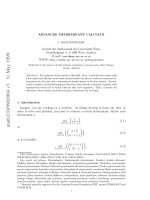
Figure 0.1: A Microscopic View of the Tangent
Copyright
c
1997 by Academic Press, Inc. - All rights reserved.
Typeset with A
M
S-T
E
X
i
Preface to the Mathematical Background
We want you to reason with mathematics. We are not trying to get everyone to give
formalized proofs in the sense of contemporary mathematics; ‘proof’ in this course means
‘convincing argument.’ We expect you to use correct reasoning and to give careful expla-
nations. The projects bring out these issues in the way we find best for most students,
but the pure mathematical questions also interest some students. This book of mathemat-
ical “background” shows how to fill in the mathematical details of the main topics from

the course. These proofs are completely rigorous in the sense of modern mathematics –
technically bulletproof. We wrote this book of foundations in part to provide a convenient
reference for a student who might like to see the “theorem - proof” approach to calculus.
We also wrote it for the interested instructor. In re-thinking the presentation of beginning
calculus, we found that a simpler basis for the theory was both possible and desirable. The
pointwise approach most books give to the theory of derivatives spoils the subject. Clear
simple arguments like the proof of the Fundamental Theorem at the start of Chapter 5 below
are not possible in that approach. The result of the pointwise approach is that instructors
feel they have to either be dishonest with students or disclaim good intuitive approximations.
This is sad because it makes a clear subject seem obscure. It is also unnecessary – by and
large, the intuitive ideas work provided your notion of derivative is strong enough. This
book shows how to bridge the gap between intuition and technical rigor.
A function with a positive derivative ought to be increasing. After all, the slope is
positive and the graph is supposed to look like an increasing straight line. How could the
function NOT be increasing? Pointwise derivatives make this bizarre thing possible - a
positive “derivative” of a non-increasing function. Our conclusion is simple. That definition
is WRONG in the sense that it does NOT support the intended idea.
You might agree that the counterintuitive consequences of pointwise derivatives are un-
fortunate, but are concerned that the traditional approach is more “general.” Part of the
point of this book is to show students and instructors that nothing of interest is lost and a
great deal is gained in the straightforward nature of the proofs based on “uniform” deriva-
tives. It actually is not possible to give a formula that is pointwise differentiable and not
uniformly differentiable. The pieced together pointwise counterexamples seem contrived
and out-of-place in a course where students are learning valuable new rules. It is a theorem
that derivatives computed by rules are automatically continuous where defined. We want
the course development to emphasize good intuition and positive results. This background
shows that the approach is sound.
This book also shows how the pathologies arise in the traditional approach – we left
pointwise pathology out of the main text, but present it here for the curious and for com-
parison. Perhaps only math majors ever need to know about these sorts of examples, but

they are fun in a negative sort of way.
This book also has several theoretical topics that are hard to find in the literature. It
includes a complete self-contained treatment of Robinson’s modern theory of infinitesimals,
first discovered in 1961. Our simple treatment is due to H. Jerome Keisler from the 1970’s.
Keisler’s elementary calculus using infinitesimals is sadly out of print. It used pointwise
derivatives, but had many novel ideas, including the first modern use of a microscope to
describe the derivative. (The l’Hospital/Bernoulli calculus text of 1696 said curves consist
of infinitesimal straight segments, but I do not know if that was associated with a magni-
fying transformation.) Infinitesimals give us a very simple way to understand the uniform
ii
derivatives, although this can also be clearly understood using function limits as in the text
by Lax, et al, from the 1970s. Modern graphical computing can also help us “see” graphs
converge as stressed in our main materials and in the interesting Uhl, Porta, Davis, Calculus
& Mathematica text.
Almost all the theorems in this book are well-known old results of a carefully studied
subject. The well-known ones are more important than the few novel aspects of the book.
However, some details like the converse of Taylor’s theorem – both continuous and discrete –
are not so easy to find in traditional calculus sources. The microscope theorem for differential
equations does not appear in the literature as far as we know, though it is similar to research
work of Francine and Marc Diener from the 1980s.
We conclude the book with convergence results for Fourier series. While there is nothing
novel in our approach, these results have been lost from contemporary calculus and deserve
to be part of it. Our development follows Courant’s calculus of the 1930s giving wonderful
results of Dirichlet’s era in the 1830s that clearly settle some of the convergence mysteries
of Euler from the 1730s. This theory and our development throughout is usually easy to
apply. “Clean” theory should be the servant of intuition – building on it and making it
stronger and clearer.
There is more that is novel about this “book.” It is free and it is not a “book” since it is
not printed. Thanks to small marginal cost, our publisher agreed to include this electronic
text on CD at no extra cost. We also plan to distribute it over the world wide web. We

hope our fresh look at the foundations of calculus will stimulate your interest. Decide for
yourself what’s the best way to understand this wonderful subject. Give your own proofs.
Contents
Part 1
Numbers and Functions
Chapter 1. Numbers 3
1.1 Field Axioms 3
1.2 Order Axioms 6
1.3 The Completeness Axiom 7
1.4 Small, Medium and Large Numbers 9
Chapter 2. Functional Identities 17
2.1 Specific Functional Identities 17
2.2 General Functional Identities 18
2.3 The Function Extension Axiom 21
2.4 Additive Functions 24
2.5 The Motion of a Pendulum 26
Part 2
Limits
Chapter 3. The Theory of Limits 31
3.1 Plain Limits 32
3.2 Function Limits 34
3.3 Computation of Limits 37
Chapter 4. Continuous Functions 43
4.1 Uniform Continuity 43
4.2 The Extreme Value Theorem 44
iii
iv Contents
4.3 Bolzano’s Intermediate Value Theorem 46
Part 3
1 Variable Differentiation

Chapter 5. The Theory of Derivatives 49
5.1 The Fundamental Theorem: Part 1 49
5.1.1 Rigorous Infinitesimal Justification 52
5.1.2 Rigorous Limit Justification 53
5.2 Derivatives, Epsilons and Deltas 53
5.3 Smoothness ⇒ Continuity of Function and Derivative 54
5.4 Rules ⇒ Smoothness 56
5.5 The Increment and Increasing 57
5.6 Inverse Functions and Derivatives 58
Chapter 6. Pointwise Derivatives 69
6.1 Pointwise Limits 69
6.2 Pointwise Derivatives 72
6.3 Pointwise Derivatives Aren’t Enough for Inverses 76
Chapter 7. The Mean Value Theorem 79
7.1 The Mean Value Theorem 79
7.2 Darboux’s Theorem 83
7.3 Continuous Pointwise Derivatives are Uniform 85
Chapter 8. Higher Order Derivatives 87
8.1 Taylor’s Formula and Bending 87
8.2 Symmetric Differences and Taylor’s Formula 89
8.3 Approximation of Second Derivatives 91
8.4 The General Taylor Small Oh Formula 92
8.4.1 The Converse of Taylor’s Theorem 95
8.5 Direct Interpretation of Higher Order Derivatives 98
8.5.1 Basic Theory of Interpolation 99
8.5.2 Interpolation where f is Smooth 101
8.5.3 Smoothness From Differences 102
Part 4
Integration
Chapter 9. Basic Theory of the Definite Integral 109

9.1 Existence of the Integral 110
Contents v
9.2 You Can’t Always Integrate Discontinuous Functions 114
9.3 Fundamental Theorem: Part 2 116
9.4 Improper Integrals 119
9.4.1 Comparison of Improper Integrals 121
9.4.2 A Finite Funnel with Infinite Area? 123
Part 5
Multivariable Differentiation
Chapter 10. Derivatives of Multivariable Functions 127
Part 6
Differential Equations
Chapter 11. Theory of Initial Value Problems 131
11.1 Existence and Uniqueness of Solutions 131
11.2 Local Linearization of Dynamical Systems 135
11.3 Attraction and Repulsion 141
11.4 Stable Limit Cycles 143
Part 7
Infinite Series
Chapter 12. The Theory of Power Series 147
12.1 Uniformly Convergent Series 149
12.2 Robinson’s Sequential Lemma 151
12.3 Integration of Series 152
12.4 Radius of Convergence 154
12.5 Calculus of Power Series 156
Chapter 13. The Theory of Fourier Series 159
13.1 Computation of Fourier Series 160
13.2 Convergence for Piecewise Smooth Functions 167
13.3 Uniform Convergence for Continuous Piecewise Smooth Functions 173
13.4 Integration of Fourier Series 175

-4 -2 2 4
w
-4
-2
2
4
x
Part 1
Numbers and Functions
2
CHAPTER
1
Numbers
This chapter gives the algebraic laws of the number systems used
in calculus.
Numbers represent various idealized measurements. Positive integers may count items,
fractions may represent a part of an item or a distance that is part of a fixed unit. Distance
measurements go beyond rational numbers as soon as we consider the hypotenuse of a right
triangle or the circumference of a circle. This extension is already in the realm of imagined
“perfect” measurements because it corresponds to a perfectly straight-sided triangle with
perfect right angle, or a perfectly round circle. Actual real measurements are always rational
and have some error or uncertainty.
The various “imaginary” aspects of numbers are very useful fictions. The rules of com-
putation with perfect numbers are much simpler than with the error-containing real mea-
surements. This simplicity makes fundamental ideas clearer.
Hyperreal numbers have ‘teeny tiny numbers’ that will simplify approximation estimates.
Direct computations with the ideal numbers produce symbolic approximations equivalent
to the function limits needed in differentiation theory (that the rules of Theorem 1.12 give
a direct way to compute.) Limit theory does not give the answer, but only a way to justify
it once you have found it.

1.1 Field Axioms
The laws of algebra follow from the field axioms. This means that algebra
is the same with Dedekind’s “real” numbers, the complex numbers, and
Robinson’s “hyperreal” numbers.
3
41.Numbers
Axiom 1.1. Field Axioms
A “field” of numbers is any set of objects together with two operations, addition
and multiplication where the operations satisfy:
• The commutative laws of addition and multiplication,
a
1
+ a
2
= a
2
+ a
1
& a
1
· a
2
= a
2
· a
1
• The associative laws of addition and multiplication,
a
1
+(a

2
+a
3
)=(a
1
+a
2
)+a
3
& a
1
·(a
2
·a
3
)=(a
1
·a
2
)·a
3
•The distributive law of multiplication over addition,
a
1
· (a
2
+ a
3
)=a
1

·a
2
+a
1
·a
3
•There is an additive identity, 0,with0+a=a for every number a.
• There is an multiplicative identity, 1,with1·a=afor every number a =0.
•Each number a has an additive inverse, −a,witha+(−a)=0.
•Each nonzero number a has a multiplicative inverse,
1
a
,witha·
1
a
=1.
A computation needed in calculus is
Example 1.1. The Cube of a Binomial
(x +∆x)
3
=x
3
+3x
2
∆x+3x∆x
2
+∆x
3
=x
3

+3x
2
∆x+(∆x(3x +∆x)) ∆x
We analyze the term ε =(∆x(3x +∆x)) in differentiation.
The reader could laboriously demonstrate that only the field axioms are needed to perform
the computation. This means it holds for rational, real, complex, or hyperreal numbers.
Here is a start. Associativity is needed so that the cube is well defined, or does not depend
on the order we multiply. We use this in the next computation, then use the distributive
property, the commutativity and the distributive property again, and so on.
(x +∆x)
3
=(x+∆x)(x +∆x)(x +∆x)
=(x+∆x)((x +∆x)(x +∆x))
=(x+∆x)((x +∆x)x+(x+∆x)∆x)
=(x+∆x)((x
2
+ x∆x)+(x∆x+∆x
2
))
=(x+∆x)(x
2
+ x∆x + x∆x +∆x
2
)
=(x+∆x)(x
2
+2x∆x+∆x
2
)
=(x+∆x)x

2
+(x+∆x)2x∆x +(x+∆x)∆x
2
)
.
.
.
The natural counting numbers 1, 2, 3, have operations of addition and multiplication,
but do not satisfy all the properties needed to be a field. Addition and multiplication do
satisfy the commutative, associative, and distributive laws, but there is no additive inverse
Field Axioms 5
0 in the counting numbers. In ancient times, it was controversial to add this element that
could stand for counting nothing, but it is a useful fiction in many kinds of computations.
The negative integers −1, −2, −3, are another idealization added to the natural num-
bers that make additive inverses possible - they are just new numbers with the needed
property. Negative integers have perfectly concrete interpretations such as measurements
to the left, rather than the right, or amounts owed rather than earned.
The set of all integers; positive, negative, and zero, still do not form a field because there
are no multiplicative inverses. Fractions, ±1/2, ±1/3, are the needed additional inverses.
When they are combined with the integers through addition, we have the set of all rational
numbers of the form ±p/q for natural numbers p and q = 0. The rational numbers are a
field, that is, they satisfy all the axioms above. In ancient times, rationals were sometimes
considered only “operators” on “actual” numbers like 1, 2, 3,
The point of the previous paragraphs is simply that we often extend one kind of number
system in order to have a new system with useful properties. The complex numbers extend
the field axioms above beyond the “real” numbers by adding a number i that solves the
equation x
2
= −1. (See the CD Chapter 29 of the main text.) Hundreds of years ago this
number was controversial and is still called “imaginary.” In fact, all numbers are useful

constructs of our imagination and some aspects of Dedekind’s “real” numbers are much
more abstract than i
2
= −1. (For example, since the reals are “uncountable,” “most” real
numbers have no description what-so-ever.)
The rationals are not “complete” in the sense that the linear measurement of the side
of an equilateral right triangle (
√
2) cannot be expressed as p/q for p and q integers. In
Section 1.3 we “complete” the rationals to form Dedekind’s “real” numbers. These numbers
correspond to perfect measurements along an ideal line with no gaps.
The complex numbers cannot be ordered with a notion of “smaller than” that is compat-
ible with the field operations. Adding an “ideal” number to serve as the square root of −1is
not compatible with the square of every number being positive. When we make extensions
beyond the real number system we need to make choices of the kind of extension depending
on the properties we want to preserve.
Hyperreal numbers allow us to compute estimates or limits directly, rather than making
inverse proofs with inequalities. Like the complex extension, hyperreal extension of the reals
loses a property; in this case completeness. Hyperreal numbers are explained beginning in
Section 1.4 below and then are used extensively in this background book to show how many
intuitive estimates lead to simple direct proofs of important ideas in calculus.
The hyperreal numbers (discovered by Abraham Robinson in 1961) are still controver-
sial because they contain infinitesimals. However, they are just another extended modern
number system with a desirable new property. Hyperreal numbers can help you understand
limits of real numbers and many aspects of calculus. Results of calculus could be proved
without infinitesimals, just as they could be proved without real numbers by using only
rationals. Many professors still prefer the former, but few prefer the latter. We believe that
is only because Dedekind’s “real” numbers are more familiar than Robinson’s, but we will
make it clear how both approaches work as a theoretical background for calculus.
There is no controversy concerning the logical soundness of hyperreal numbers. The use

of infinitesimals in the early development of calculus beginning with Leibniz, continuing with
Euler, and persisting to the time of Gauss was problematic. The founders knew that their
use of infinitesimals was logically incomplete and could lead to incorrect results. Hyperreal
numbers are a correct treatment of infinitesimals that took nearly 300 years to discover.
61.Numbers
With hindsight, they also have a simple description. The Function Extension Axiom 2.1
explained in detail in Chapter 2 was the missing key.
Exercise set 1.1
1. Show that the identity numbers 0 and 1 are unique. (HINT: Suppose 0

+ a = a.Add
−ato both sides.)
2. Show that 0 ·a =0. (HINT: Expand

0+
b
a

·a with the distributive law and show that
0 ·a + b = b. Then use the previous exercise.)
3. The inverses −a and
1
a
are unique. (HINT: Suppose not, 0=a−a=a+b.Add−a
to both sides and use the associative property.)
4. Show that −1 ·a = −a. (HINT: Use the distributive property on 0=(1−1) ·a and use
the uniqueness of the inverse.)
5. Show that (−1) ·(−1) = 1.
6. Other familiar properties of algebra follow from the axioms, for example, if a
3

=0and
a
4
=0,then
a
1
+a
2
a
3
=
a
1
a
3
+
a
2
a
3
,
a
1
·a
2
a
3
·a
4
=

a
1
a
3
·
a
2
a
4
& a
3
·a
4
=0
1.2 Order Axioms
Estimation is based on the inequality ≤ oftherealnumbers.
One important representation of rational and real numbers is as measurements of distance
along a line. The additive identity 0 is located as a starting point and the multiplicative
identity 1 is marked off (usually to the right on a horizontal line). Distances to the right
correspond to positive numbers and distances to the left to negative ones. The inequality
< indicates which numbers are to the left of others. The abstract properties are as follows.
Axiom 1.2. Ordered Field Axioms
A a number system is an ordered field if it satisfies the field Axioms 1.1 and has a
relation < that satisfies:
• Every pair of numbers a and b satisfies exactly one of the relations
a = b, a<b,orb<a
•If a<band b<c,thena<c.
•If a<b,thena+c<b+c.
•If 0 <aand 0 <b,then0<a·b.
These axioms have simple interpretations on the number line. The first order axiom says

that every two numbers can be compared; either two numbers are equal or one is to the left
of the other.
The Completeness Axiom 7
The second axiom, called transitivity, says that if a is left of b and b is left of c,thenais
left of c.
The third axiom says that if a is left of b and we move both by a distance c, then the
results are still in the same left-right order.
The fourth axiom is the most difficult abstractly. All the compatibility with multiplication
is built from it.
The rational numbers satisfy all these axioms, as do the real and hyperreal numbers. The
complex numbers cannot be ordered in a manner compatible with the operations of addition
and multiplication.
Definition 1.3. Absolute Value
If a is a nonzero number in an ordered field, |a| is the larger of a and −a, that is,
|a| = a if −a<aand |a| = −a if a<−a.Welet|0|=0.
Exercise set 1.2
1. If 0 <a, show that −a<0by using the additive property.
2. Show that 0 < 1. (HINT: Recall the exercise that (−1) ·(−1) = 1 and argue by contra-
diction, supposing 0 < −1.)
3. Show that a · a>0for every a =0.
4. Show that there is no order < on the complex numbers that satisfies the ordered field
axioms.
5. Prove that if a<band c>0,thenc·a<c·b.
Prove that if 0 <a<band 0 <c<d,thenc·a<d·b.
1.3 The Completeness Axiom
Dedekind’s “real” numbers represent points on an ideal line with no gaps.
The number
√
2 is not rational. Suppose to the contrary that
√

2=q/r for integers q
and r with no common factors. Then 2r
2
= q
2
. The prime factorization of both sides must
be the same, but the factorization of the squares have an even number distinct primes on
each side and the 2 factor is left over. This is a contradiction, so there is no rational number
whose square is 2.
A length corresponding to
√
2 can be approximated by (rational) decimals in various
ways, for example, 1 < 1.4 < 1.41 < 1.414 < 1.4142 < 1.41421 < 1.414213 < There
is no rational for this sequence to converge to, even though it is “trying” to converge. For
example, all the terms of the sequence are below 1.41422 < 1.4143 < 1.415 < 1.42 < 1.5 < 2.
Even without remembering a fancy algorithm for finding square root decimals, you can test
81.Numbers
the successive decimal approximations by squaring, for example, 1.41421
2
=1.9999899241
and 1.41422
2
=2.0000182084.
It is perfectly natural to add a new number to the rationals to stand for the limit of
the better and better approximations to
√
2. Similarly, we could devise approximations
to π and make π the number that stands for the limit of such successive approximations.
We would like a method to include “all such possible limits” without having to specify the
particular approximations. Dedekind’s approach is to let the real numbers be the collection

of all “cuts” on the rational line.
Definition 1.4. A Dedekind Cut
A “cut” in an ordered field is a pair of nonempty sets A and B so that:
• Every number is either in A or B.
• Every a in A is less than every b in B.
We may think of
√
2 defining a cut of the rational numbers where A consists of all rational
numbers a with a<0ora
2
<2andBconsists of all rational numbers b with b
2
> 2. There
is a “gap” in the rationals where we would like to have
√
2. Dedekind’s “real numbers” fill
all such gaps. In this case, a cut of real numbers would have to have
√
2 either in A or in
B.
Axiom 1.5. Dedekind Completeness
The real numbers are an ordered field such that if A and B form a cut in those
numbers, there is a number r such that r is in either A or in B and all other the
numbers in A satisfy a<rand in B satisfy r<b.
In other words, every cut on the “real” line is made at some specific number r,sothere
are no gaps. This seems perfectly reasonable in cases like
√
2andπwhere we know specific
ways to describe the associated cuts. The only drawback to Dedekind’s number system
is that “every cut” is not a very concrete notion, but rather relies on an abstract notion

of “every set.” This leads to some paradoxical facts about cuts that do not have specific
descriptions, but these need not concern us. Every specific cut has a real number in the
middle.
Completeness of the reals means that “approximation procedures” that are “improving”
converge to a number. We need to be more specific later, but for example, bounded in-
creasing or decreasing sequences converge and “Cauchy” sequences converge. We will not
describe these details here, but take them up as part of our study of limits below.
Completeness has another important consequence, the Archimedean Property Theo-
rem 1.8. We take that up in the next section. The Archimedean Property says precisely that
the real numbers contain no positive infinitesimals. Hyperreal numbers extend the reals by
including infinitesimals. (As a consequence the hyperreals are not Dedekind complete.)
Small, Medium and Large Numbers 9
1.4 Small, Medium and Large Num-
bers
Hyperreal numbers give us a way to simplify estimation by adding infinites-
imal numbers to the real numbers.
We want to have three different intuitive sizes of numbers, very small, medium size, and
very large. Most important, we want to be able to compute with these numbers using the
same rules of algebra as in high school and separate the ‘small’ parts of our computation.
Hyperreal numbers give us these computational estimates. Hyperreal numbers satisfy three
axioms which we take up separately below, Axiom 1.7, Axiom 1.9, and Axiom 2.1.
As a first intuitive approximation, we could think of these scales of numbers in terms of
the computer screen. In this case, ‘medium’ numbers might be numbers in the range -999 to
+ 999 that name a screen pixel. Numbers closer than one unit could not be distinguished by
different screen pixels, so these would be ‘tiny’ numbers. Moreover, two medium numbers
a and b would be indistinguishably close, a ≈ b, if their difference was a ‘tiny’ number less
than a pixel. Numbers larger in magnitude than 999 are too big for the screen and could
be considered ‘huge.’
The screen distinction sizes of computer numbers is a good analogy, but there are diffi-
culties with the algebra of screen - size numbers. We want to have ordinary rules of algebra

and the following properties of approximate equality. For now, all you should think of is
that ≈ means ‘approximately equals.’
(a) If p and q are medium, so are p + q and p ·q.
(b) If ε and δ are tiny, so is ε + δ,thatis,ε≈0andδ≈0 implies ε + δ ≈ 0.
(c) If δ ≈ 0andqis medium, then q · δ ≈ 0.
(d) 1/0 is still undefined and 1/x is huge only when x ≈ 0.
You can see that the computer number idea does not quite work, because the approximation
rules don’t always apply. If p =15.37 and q = −32.4, then p·q = −497.998 ≈−498, ‘medium
times medium is medium,’ however, if p = 888 and q = 777, then p · q is no longer screen
size
The hyperreal numbers extend the ‘real’ number system to include ‘ideal’ numbers that
obey these simple approximation rules as well as the ordinary rules of algebra and trigonom-
etry. Very small numbers technically are called infinitesimals and what we shall assume that
is different from high school is that there are positive infinitesimals.
Definition 1.6. Infinitesimal Number
Anumberδin an ordered field is called infinitesimal if it satisfies
1
2
>
1
3
>
1
4
> ···>
1
m
>···> |δ|
for any ordinary natural counting number m =1,2,3,···.Wewritea≈band say
a is infinitely close to b if the number b −a ≈ 0 is infinitesimal.

This definition is intended to include 0 as “infinitesimal.”
10 1. Numbers
Axiom 1.7. The Infinitesimal Axiom
The hyperreal numbers contain the real numbers, but also contain nonzero infinites-
imal numbers, that is, numbers δ ≈ 0, positive, δ>0, but smaller than all the real
positive numbers.
This stands in contrast to the following result.
Theorem 1.8. The Archimedean Property
The hyperreal numbers are not Dedekind complete and there are no positive in-
finitesimal numbers in the ordinary reals, that is, if r>0is a positive real number,
then there is a natural counting number m such that 0 <
1
m
<r.
Proof:
We define a cut above all the positive infinitesimals. The set A consists of all numbers a
satisfying a<1/m for every natural counting number m.ThesetBconsists of all numbers
b such that there is a natural number m with 1/m < b. The pair A, B defines a Dedekind
cut in the rationals, reals, and hyperreal numbers. If there is a positive δ in A, then there
cannot be a number at the gap. In other words, there is no largest positive infinitesimal or
smallest positive non-infinitesimal. This is clear because δ<δ+δand 2δ is still infinitesimal,
while if ε is in B, ε/2 <εmust also be in B.
Since the real numbers must have a number at the “gap,” there cannot be any positive
infinitesimal reals. Zero is at the gap in the reals and every positive real number is in B.
This is what the theorem asserts, so it is proved. Notice that we have also proved that the
hyperreals are not Dedekind complete, because the cut in the hyperreals must have a gap.
Two ordinary real numbers, a and b,satisfya≈bonly if a = b, since the ordinary real
numbers do not contain infinitesimals. Zero is the only real number that is infinitesimal.
If you prefer not to say ‘infinitesimal,’ just say ‘δ is a tiny positive number’ and think
of ≈ as ‘close enough for the computations at hand.’ The computation rules above are still

important intuitively and can be phrased in terms of limits of functions if you wish. The
intuitive rules help you find the limit.
The next axiom about the new “hyperreal” numbers says that you can continue to do
the algebraic computations you learned in high school.
Axiom 1.9. The Algebra Axiom (Including < rules.)
The hyperreal numbers are an ordered field, that is, they obey the same rules of
ordered algebra as the real numbers, Axiom 1.1 and Axiom 1.2.
The algebra of infinitesimals that you need can be learned by working the examples and
exercises in this chapter.
Functional equations like the addition formulas for sine and cosine or the laws of logs
and exponentials are very important. (The specific high school identities are reviewed in
the main text CD Chapter 28 on High School Review.) The Function Extension Axiom 2.1
shows how to extend the non-algebraic parts of high school math to hyperreal numbers.
This axiom is the key to Robinson’s rigorous theory of infinitesimals and it took 300 years
to discover. You will see by working with it that it is a perfectly natural idea, as hindsight
often reveals. We postpone that to practice with the algebra of infinitesimals.
Example 1.2. The Algebra of Small Quantities
Small, Medium and Large Numbers 11
Let’s re-calculate the increment of the basic cubic using the new numbers. Since the rules
of algebra are the same, the same basic steps still work (see Example 1.1), except now we
may take x any number and δx an infinitesimal.
Small Increment of f[x]=x
3
f[x+δx]=(x+δx)
3
= x
3
+3x
2
δx +3xδx

2
+ δx
3
f[x + δx]=f[x]+3x
2
δx +(δx[3x + δx]) δx
f[x + δx]=f[x]+f

[x]δx + εδx
with f

[x]=3x
2
and ε =(δx[3x + δx]). The intuitive rules above show that ε ≈ 0 whenever
x is finite. (See Theorem 1.12 and Example 1.8 following it for the precise rules.)
Example 1.3. Finite Non-Real Numbers
The hyperreal numbers obey the same rules of algebra as the familiar numbers from high
school. We know that r+∆ >r, whenever ∆ > 0 is an ordinary positive high school number.
(See the addition property of Axiom 1.2.) Since hyperreals satisfy the same rules of algebra,
we also have new finite numbers given by a high school number r plus an infinitesimal,
a = r + δ>r
The number a = r + δ is different from r, even though it is infinitely close to r. Since δ is
small, the difference between a and r is small
0 <a−r=δ≈0ora≈rbut a = r
Here is a technical definition of “finite” or “limited” hyperreal number.
Definition 1.10. Limited and Unlimited Hyperreal Numbers
A hyperreal number x is said to be finite (or limited) if there is an ordinary natural
number m =1,2,3,··· so that
|x| <m.
If a number is not finite, we say it is infinitely large (or unlimited).

Ordinary real numbers are part of the hyperreal numbers and they are finite because
they are smaller than the next integer after them. Moreover, every finite hyperreal number
is near an ordinary real number (see Theorem 1.11 below), so the previous example is the
most general kind of finite hyperreal number there is. The important thing is to learn to
compute with approximate equalities.
Example 1.4. A Magnified View of the Hyperreal Line
Of course, infinitesimals are finite, since δ ≈ 0 implies that |δ| < 1. The finite numbers are
not just the ordinary real numbers and the infinitesimals clustered near zero. The rules of
algebra say that if we add or subtract a nonzero number from another, the result is a different
number. For example, π −δ<π<π+δ,when0<δ≈0. These are distinct finite hyperreal
numbers but each of these numbers differ by only an infinitesimal, π ≈ π + δ ≈ π − δ.If
we plotted the hyperreal number line at unit scale, we could only put one dot for all three.
However, if we focus a microscope of power 1/δ at π we see three points separated by unit
distances.
12 1. Numbers
X 1/d
Pi
Pi + d
Pi - d
Figure 1.1: Magnification at Pi
The basic fact is that finite numbers only differ from reals by an infinitesimal. (This is
equivalent to Dedekind’s Completeness Axiom.)
Theorem 1.11. Standard Parts of Finite Numbers
Every finite hyperreal number x differs from some ordinary real number r by an
infinitesimal amount, x−r ≈ 0 or x ≈ r. The ordinary real number infinitely near
x is called the standard part of x, r =st(x).
Proof:
Suppose x is a finite hyperreal. Define a cut in the real numbers by letting A be the
set of all real numbers satisfying a ≤ x and letting B be the set of all real numbers b with
x<b.BothAand B are nonempty because x is finite. Every a in A is below every b

in B by transitivity of the order on the hyperreals. The completeness of the real numbers
means that there is a real r at the gap between A and B.Wemusthavex≈r, because if
x −r>1/m,say,thenr+1/(2m) <xand by the gap property would need to be in B.
A picture of the hyperreal number line looks like the ordinary real line at unit scale.
We can’t draw far enough to get to the infinitely large part and this theorem says each
finite number is indistinguishably close to a real number. If we magnify or compress by new
number amounts we can see new structure.
You still cannot divide by zero (that violates rules of algebra), but if δ is a positive
infinitesimal, we can compute the following:
−δ, δ
2
,
1
δ
What can we say about these quantities?
The idealization of infinitesimals lets us have our cake and eat it too. Since δ =0,we
can divide by δ. However, since δ is tiny, 1/δ must be HUGE.
Example 1.5. Negative infinitesimals
In ordinary algebra, if ∆ > 0, then −∆ < 0, so we can apply this rule to the infinitesimal
number δ and conclude that −δ<0, since δ>0.
Example 1.6. Orders of infinitesimals
In ordinary algebra, if 0 < ∆ < 1, then 0 < ∆
2
< ∆, so 0 <δ
2
<δ.
We want you to formulate this more exactly in the next exercise. Just assume δ is
very small, but positive. Formulate what you want to draw algebraically. Try some small
ordinary numbers as examples, like δ =0.01. Plot δ at unit scale and place δ
2

accurately
on the figure.
Example 1.7. Infinitely large numbers
Small, Medium and Large Numbers 13
For real numbers if 0 < ∆ < 1/n then n<1/∆. Since δ is infinitesimal, 0 <δ<1/n
for every natural number n =1,2,3, Using ordinary rules of algebra, but substituting
the infinitesimal δ,weseethatH=1/δ > n is larger than any natural number n (or is
“infinitely large”), that is, 1 < 2 < 3 < <n<H, for every natural number n.Wecan
“see” infinitely large numbers by turning the microscope around and looking in the other
end.
The new algebraic rules are the ones that tell us when quantities are infinitely close,
a ≈ b. Such rules, of course, do not follow from rules about ordinary high school numbers,
but the rules are intuitive and simple. More important, they let us ‘calculate limits’ directly.
Theorem 1.12. Computation Rules for Finite and Infinitesimal Numbers
(a) If p and q arefinite,soarep+qand p ·q.
(b) If ε and δ are infinitesimal, so is ε + δ.
(c) If δ ≈ 0 and q is finite, then q · δ ≈ 0. (finite x infsml = infsml)
(d) 1/0 is still undefined and 1/x is infinitely large only when x ≈ 0.
To understand these rules, just think of p and q as “fixed,” if large, and δ as being as
small as you please (but not zero). It is not hard to give formal proofs from the definitions
above, but this intuitive understanding is more important. The last rule can be “seen” on
the graph of y =1/x. Look at the graph and move down near the values x ≈ 0.
x
y
Figure 1.2: y =1/x
Proof:
We prove rule (c) and leave the others to the exercises. If q is finite, there is a natural
number m so that |q| <m. We want to show that |q · δ| < 1/n for any natural number n.
Since δ is infinitesimal, we have |δ| < 1/(n ·m). By Exercise 1.2.5, |q|·|δ|<m·
1

n·m
=
1
m
.
Example 1.8. y = x
3
⇒ dy =3x
2
dx, for finite x
The error term in the increment of f[x]=x
3
, computed above is
ε =(δx[3x + δx])
If x is assumed finite, then 3x is also finite by the first rule above. Since 3x and δx are finite,
so is the sum 3x + δx by that rule. The third rule, that says an infinitesimal times a finite
number is infinitesimal, now gives δx× finite = δx[3x + δx] = infinitesimal, ε ≈ 0. This
14 1. Numbers
justifies the local linearity of x
3
at finite values of x, that is, we have used the approximation
rules to show that
f[x + δx]=f[x]+f

[x] δx + εδx
with ε ≈ 0 whenever δx ≈ 0andxis finite, where f[x]=x
3
and f

[x]=3x

2
.
Exercise set 1.4
1. Draw the view of the ideal number line when viewed under an infinitesimal microscope
of power 1/δ. Which number appears unit size? How big does δ
2
appear at this scale?
Where do the numbers δ and δ
3
appear on a plot of magnification 1/δ
2
?
2. Backwards microscopes or compression
Draw the view of the new number line when viewed under an infinitesimal microscope
with its magnification reversed to power δ (not 1/δ). What size does the infinitely large
number H (HUGE) appear to be? What size does the finite (ordinary) number m =10
9
appear to be? Can you draw the number H
2
on the plot?
3. y = x
p
⇒ dy = px
p−1
dx, p =1,2,3,
For each f [x]=x
p
below:
(a) Compute f[x + δx] −f[x] and simplify, writing the increment equation:
f[x + δx] −f[x]=f


[x]·δx + ε ·δx
=[term in x but not δx]δx +[observed microscopic error]δx
Notice that we can solve the increment equation for ε =
f[x + δx] −f[x]
δx
−f

[x]
(b) Show that ε ≈ 0 if δx ≈ 0 and x is finite. Does x need to be finite, or can it be
any hyperreal number and still have ε ≈ 0?
(1) If f[x]=x
1
,thenf

[x]=1x
0
=1and ε =0.
(2) If f[x]=x
2
,thenf

[x]=2xand ε = δx.
(3) If f[x]=x
3
,thenf

[x]=3x
2
and ε =(3x+δx)δx.

(4) If f[x]=x
4
,thenf

[x]=4x
3
and ε =(6x
2
+4xδx + δx
2
)δx.
(5) If f[x]=x
5
,thenf

[x]=5x
4
and ε =(10x
3
+10x
2
δx +5xδx
2
+ δx
3
)δx.
4. Exceptional Numbers and the Derivative of y =
1
x
(a) Let f [x]=1/x and show that

f[x + δx] −f[x]
δx
=
−1
x(x + δx)
(b) Compute
ε =
−1
x(x + δx)
+
1
x
2
= δx ·
1
x
2
(x + δx)
(c) Show that this gives
f[x + δx] −f[x]=f

[x]·δx + ε ·δx
when f

[x]=−1/x
2
.
(d) Show that ε ≈ 0 provided x is NOT infinitesimal (and in particular is not zero.)
Small, Medium and Large Numbers 15
5. Exceptional Numbers and the Derivative of y =

√
x
(a) Let f [x]=
√
xand compute
f[x + δx] −f[x]=
1
√
x+δx +
√
x
(b) Compute
ε =
1
√
x + δx +
√
x
−
1
2
√
x
=
−1
2
√
x(
√
x + δx +

√
x)
2
·δx
(c) Show that this gives
f[x + δx] −f[x]=f

[x]·δx + ε ·δx
when f

[x]=
1
2
√
x
.
(d) Show that ε ≈ 0 provided x is positive and NOT infinitesimal (and in particular
is not zero.)
6. Prove the remaining parts of Theorem 1.12.
16 1. Numbers
CHAPTER
2
Functional Identities
In high school you learned that trig functions satisfy certain iden-
tities or that logarithms have certain “properties.” This chapter
extends the idea of functional identities from specific cases to a
defining property of an unknown function.
The use of “unknown functions” is of fundamental importance in calculus, and other
branches of mathematics and science. For example, differential equations can be viewed as
identities for unknown functions.

One reason that students sometimes have difficulty understanding the meaning of deriva-
tives or even the general rules for finding derivatives is that those things involve equations in
unknown functions. The symbolic rules for differentiation and the increment approximation
defining derivatives involve unknown functions. It is important for you to get used to this
“higher type variable,” an unknown function. This chapter can form a bridge between the
specific identities of high school and the unknown function variables from rules of calculus
and differential equations.
2.1 Specific Functional Identities
All the the identities you need to recall from high school are:
(Cos[x])
2
+ (Sin[x])
2
= 1 CircleIden
Cos[x + y]=Cos[x]Cos[y]−Sin[x] Sin[y] CosSum
Sin[x + y] = Sin[x]Cos[y] + Sin[y]Cos[x] SinSum
b
x+y
= b
x
b
y
ExpSum
(b
x
)
y
= b
x·y
RepeatedExp

Log[x · y] = Log[x]+Log[y] LogProd
Log[x
p
]=pLog[x] LogPower
but you must be able to use these identities. Some practice exercises using these familiar
identities are given in main text CD Chapter 28.
17
18 2. Functional Identities
2.2 General Functional Identities
A general functional identity is an equation which is satisfied by an unknown
function (or a number of functions) over its domain.
The function
f[x]=2
x
satisfies f[x + y]=2
(x+y)
=2
x
2
y
=f[x]f[y], so eliminating the two middle terms, we see
that the function f [x]=2
x
satisfies the functional identity
f[x + y]=f[x]f[y](ExpSum)
It is important to pay attention to the variable or variables in a functional identity. In order
for an equation involving a function to be a functional identity, the equation must be valid for
all values of the variables in question. Equation (ExpSum) above is satisfied by the function
f[x]=2
x

for all x and y. For the function f [x]=x,itistruethatf[2 + 2] = f[2]f [2], but
f[3 + 1] = f[3]f[1], so = x does not satisfy functional identity (ExpSum).
Functional identities are a sort of ‘higher laws of algebra.’ Observe the notational simi-
larity between the distributive law for multiplication over addition,
m ·(x + y)=m·x+m·y
and the additive functional identity
f[x + y]=f[x]+f[y](Additive)
Most functions f [x] do not satisfy the additive identity. For example,
1
x + y
=
1
x
+
1
y
and
√
x + y =
√
x +
√
y
The fact that these are not identities means that for some choices of x and y in the domains
of the respective functions f[x]=1/x and f[x]=
√
x, the two sides are not equal. You
will show below that the only differentiable functions that do satisfy the additive functional
identity are the functions f[x]=m·x. In other words, the additive functional identity is
nearly equivalent to the distributive law; the only unknown (differentiable) function that

satisfies it is multiplication. Other functional identities such as the 7 given at the start of
this chapter capture the most important features of the functions that satisfy the respective
identities. For example, the pair of functions f[x]=1/x and g[x]=
√
xdo not satisfy the
addition formula for the sine function, either.
Example 2.1. The Microscope Equation
The “microscope equation” defining the differentiability of a function f[x] (see Chapter
5 of the text),
f[x + δx]=f[x]+f

[x]·δx + ε ·δx(Micro)
General Functional Identities 19
with ε ≈ 0ifδx ≈ 0, is similar to a functional identity in that it involves an unknown
function f[x] and its related unknown derivative function f

[x]. It “relates” the function
f[x] to its derivative
df
dx
= f

[x].
You should think of (Micro) as the definition of the derivative of f[x]atagivenx, but
also keep in mind that (Micro) is the definition of the derivative of any function. If we let
f[x] vary over a number of different functions, we get different derivatives. The equation
(Micro) can be viewed as an equation in which the function, f [x], is the variable input, and
the output is the derivative
df
dx

.
To make this idea clearer, we rewrite (Micro) by solving for
df
dx
:)
df
dx
=
f[x + δx] −f[x]
δx
−ε
or
df
dx
= lim
∆x→0
f[x + δx] −f[x]
∆x
If we plug in the “input” function f[x]=x
2
into this equation, the output is
df
dx
=2x.Ifwe
plug in the “input” function f[x] = Log[x], the output is
df
dx
=
1
x

. The microscope equation
involves unknown functions, but strictly speaking, it is not a functional identity, because
of the error term ε (or the limit which can be used to formalize the error). It is only an
approximate identity.
Example 2.2. Rules of Differentiation
The various “differentiation rules,” the Superposition Rule, the Product Rule and the
Chain Rule (from Chapter 6 of the text) are functional identities relating functions and
their derivatives. For example, the Product Rule states:
d(f[x]g[x])
dx
=
df
dx
g[x]+f[x]
dg
dx
We can think of f[x]andg[x] as “variables” which vary by simply choosing different actual
functions for f[x]andg[x]. Then the Product Rule yields an identity between the choices
of f [x]andg[x], and their derivatives. For example, choosing f [x]=x
2
and g[x] = Log[x]
and plugging into the Product Rule yields
d(x
2
Log[x])
dx
=2xLog[x]+x
2
1
x

Choosing f[x]=x
3
and g[x]=Exp[x] and plugging into the Product Rule yields
d(x
3
Exp[x])
dx
=3x
2
Exp[x]+x
3
Exp[x]
If we choose f[x]=x
5
, but do not make a specific choice for g[x], plugging into the
Product Rule will yield
d(x
5
g[x])
dx
=5x
4
g[x]+x
5
dg
dx
The goal of this chapter is to extend your thinking to identities in unknown functions.