DIRECT NUMERICAL SIMULATIONS OF GAS–LIQUID MULTIPHASE FLOWS pot
Bạn đang xem bản rút gọn của tài liệu. Xem và tải ngay bản đầy đủ của tài liệu tại đây (7.19 MB, 337 trang )
DIRECT NUMERICAL SIMULATIONS
OF GAS–LIQUID MULTIPHASE FLOWS
Accurately predicting the behavior of multiphase flows is a problem of immense
industrial and scientific interest. Using modern computers, researchers can now
study the dynamics in great detail, and computer simulations are yielding unprece-
dented insight. This book provides a comprehensive introduction to direct numer-
ical simulations of multiphase flows for researchers and graduate students.
After a brief overview of the context and history, the authors review the gov-
erning equations. A particular emphasis is placed on the “one-fluid” formulation,
where a single set of equations is used to describe the entire flow field and in-
terface terms are included as singularity distributions. Several applications are
discussed, such as atomization, droplet impact, breakup and collision, and bubbly
flows, showing how direct numerical simulations have helped researchers advance
both our understanding and our ability to make predictions. The final chapter
gives an overview of recent studies of flows with relatively complex physics, such
as mass transfer and chemical reactions, solidification, and boiling, and includes
extensive references to current work.
GR
´
ETAR TRYGGVASON is the Viola D. Hank Professor of Aerospace and
Mechanical Engineering at the University of Notre Dame, Indiana.
RUBEN SCARDOVELLI is an Associate Professor in the Dipartimento di Inge-
gneria Energetica, Nucleare e del Controllo Ambientale (DIENCA) of the Univer-
sit
`
a degli Studi di Bologna.
ST
´
EPHANE ZALESKI is a Professor of Mechanics at the Universit
´
e Pierre et
Marie Curie (UPMC) in Paris and Head of the Jean Le Rond d’Alembert Institute
(CNRS UMR 7190).
DIRECT NUMERICAL SIMULATIONS
OF GAS–LIQUID MULTIPHASE FLOWS
GR
´
ETAR TRYGGVASON
University of Notre Dame, Indiana
RUBEN SCARDOVELLI
Universit
`
a degli Studi di Bologna
ST
´
EPHANE ZALESKI
Universit
´
e Pierre et Marie Curie, Paris 6
CAMBRIDGE UNIVERSITY PRESS
Cambridge, New York, Melbourne, Madrid, Cape Town,
Singapore, S
˜
ao Paulo, Delhi, Tokyo, Mexico City
Cambridge University Press
The Edinburgh Building, Cambridge CB2 8RU, UK
Published in the United States of America by Cambridge University Press, New York
www.cambridge.org
Information on this title: www.cambridge.org/9780521782401
C
Cambridge University Press 2011
This publication is in copyright. Subject to statutory exception
and to the provisions of relevant collective licensing agreements,
no reproduction of any part may take place without the written
permission of Cambridge University Press.
First published 2011
Printed in the United Kingdom at the University Press, Cambridge
A catalogue record for this publication is available from the British Library
ISBN 978-0-521-78240-1 Hardback
Cambridge University Press has no responsibility for the persistence or
accuracy of URLs for external or third-party internet websites referred to
in this publication, and does not guarantee that any content on such
websites is, or will remain, accurate or appropriate.
Contents
Preface page ix
1 Introduction 1
1.1 Examples of multiphase flows 3
1.2 Computational modeling 7
1.3 Looking ahead 18
2 Fluid mechanics with interfaces 21
2.1 General principles 21
2.2 Basic equations 22
2.3 Interfaces: description and definitions 30
2.4 Fluid mechanics with interfaces 36
2.5 Fluid mechanics with interfaces: the one-fluid formulation 41
2.6 Nondimensional numbers 42
2.7 Thin films, intermolecular forces, and contact lines 44
2.8 Notes 47
3 Numerical solutions of the Navier–Stokes equations 50
3.1 Time integration 51
3.2 Spatial discretization 55
3.3 Discretization of the advection terms 59
3.4 The viscous terms 61
3.5 The pressure equation 64
3.6 Velocity boundary conditions 69
3.7 Outflow boundary conditions 70
3.8 Adaptive mesh refinement 71
3.9 Summary 72
3.10 Postscript: conservative versus non-conservative form 73
4 Advecting a fluid interface 75
4.1 Notations 76
v
vi Contents
4.2 Advecting the color function 77
4.3 The volume-of-fluid (VOF) method 81
4.4 Front tracking 84
4.5 The level-set method 87
4.6 Phase-field methods 90
4.7 The CIP method 91
4.8 Summary 93
5 The volume-of-fluid method 95
5.1 Basic properties 95
5.2 Interface reconstruction 98
5.3 Tests of reconstruction methods 106
5.4 Interface advection 108
5.5 Tests of reconstruction and advection methods 122
5.6 Hybrid methods 128
6 Advecting marker points: front tracking 133
6.1 The structure of the front 134
6.2 Restructuring the fronts 143
6.3 The front-grid communications 145
6.4 Advection of the front 150
6.5 Constructing the marker function 152
6.6 Changes in the front topology 158
6.7 Notes 160
7 Surface tension 161
7.1 Computing surface tension from marker functions 161
7.2 Computing the surface tension of a tracked front 168
7.3 Testing the surface tension methods 177
7.4 More sophisticated surface tension methods 181
7.5 Conclusion on numerical methods 186
8 Disperse bubbly flows 187
8.1 Introduction 187
8.2 Homogeneous bubbly flows 189
8.3 Bubbly flows in vertical channels 194
8.4 Discussion 201
9 Atomization and breakup 204
9.1 Introduction 204
9.2 Thread, sheet, and rim breakup 205
9.3 High-speed jets 214
9.4 Atomization simulations 219
Contents vii
10 Droplet collision, impact, and splashing 228
10.1 Introduction 228
10.2 Early simulations 229
10.3 Low-velocity impacts and collisions 229
10.4 More complex slow impacts 232
10.5 Corolla, crowns, and splashing impacts 235
11 Extensions 243
11.1 Additional fields and surface physics 243
11.2 Imbedded boundaries 256
11.3 Multiscale issues 266
11.4 Summary 269
Appendix A Interfaces: description and definitions 270
A.1 Two-dimensional geometry 270
A.2 Three-dimensional geometry 272
A.3 Axisymmetric geometry 274
A.4 Differentiation and integration on surfaces 275
Appendix B Distributions concentrated on the interface 279
B.1 A simple example 281
Appendix C Cube-chopping algorithm 284
C.1 Two-dimensional problem 285
C.2 Three-dimensional problem 286
Appendix D The dynamics of liquid sheets: linearized theory 288
D.1 Flow configuration 288
D.2 Inviscid results 288
D.3 Viscous theory for the Kelvin–Helmholtz instability 293
References 295
Index 322
Preface
Progress is usually a sequence of events where advances in one field open up new
opportunities in another, which in turn makes it possible to push yet another field
forward, and so on. Thus, the development of fast and powerful computers has
led to the development of new numerical methods for direct numerical simula-
tions (DNS) of multiphase flows that have produced detailed studies and improved
knowledge of multiphase flows. While the origin of DNS of multiphase flows goes
back to the beginning of computational fluid dynamics in the early sixties, it is
only in the last decade and a half that the field has taken off. We, the authors of
this book, have had the privilege of being among the pioneers in the development
of these methods and among the first researchers to apply DNS to study relatively
complex multiphase flows. We have also had the opportunity to follow the progress
of others closely, as participants in numerous meetings, as visitors to many labo-
ratories, and as editors of scientific journals such as the Journal of Computational
Physics and the International Journal of Multiphase Flows. To us, the state of the
art can be summarized by two observations:
• Even though there are superficial differences between the various approaches
being pursued for DNS of multiphase flows, the similarities and commonalities
of the approaches are considerably greater than the differences.
• As methods become more sophisticated and the problems of interest become
more complex, the barrier that must be overcome by a new investigator wishing
to do DNS of multiphase flows keeps increasing.
This book is an attempt to address both issues.
The development of numerical methods for flows containing a sharp interface,
as fluids consisting of two or more immiscible components inherently do, is cur-
rently a “hot” topic and significant progress has been made by a number of groups.
Indeed, for a while there was hardly an issue of the Journal of Computational
Physics that did not contain one or more papers describing such methods. In the
present book we have elected to focus mostly on two specific classes of methods:
volume of fluid (VOF) and front-tracking methods. This choice reflects our own
background, as well as the fact that both types of method have been very successful
and are responsible for some of the most significant new insights into multiphase
flow dynamics that DNS has revealed. Furthermore, as emphasized by the first
bullet point, the similarities in the different approaches are sufficiently great that
ix
x Preface
a reader of the present book would most likely find it relatively easy to switch to
other methods capable of capturing the interface, such as level set and phase field.
The goal of DNS of multiphase flows is the understanding of the behavior and
properties of such flows. We believe that while the development of numerical
methods is important, it is in their applications where the most significant rewards
are to be found. Thus, we include in the book several chapters where we describe
the use of DNS to understand specific systems and what has been learned up to now.
This is inherently a somewhat biased sample (since we elected to talk about studies
that we know well – our own!), but we feel that the importance of these chapters
goes beyond the specific topics treated. We furthermore firmly believe that the
methods that we describe here have now reached sufficient maturity so that they
can be used to probe the mysteries of a large number of complex flows. Therefore,
the application of existing methods to problems that they are suited for and the
development of new numerical methods for more complex flows, such as those
described in the final chapter, are among the most exciting immediate directions
for DNS of multiphase flows.
Our work has benefitted from the efforts of many colleagues and friends. First
and foremost we thank our students, postdoctoral researchers and visitors for the
many and significant contributions they have made to the work presented here. GT
would like to thank his students, Drs. D. Yu, M. Song, S.O. Unverdi, E. Ervin,
M.R. Nobari, C.H.H. Chang, Y J. Jan, S. Nas, M. Saeed, A. Esmaeeli, F. Tounsi,
D. Juric, N.C. Suresh, J. Han, J. Che, B. Bunner, N. Al-Rawahi, W. Tauber, M.
Stock, S. Biswas, and S. Thomas, as well as the following visitors and postdoctoral
researchers: S. Homma, J. Wells, A. Fernandez, and J. Lu. RS would like to thank
his students, Drs. E. Aulisa, L. Campioni, A. Cervone, and V. Marra, as well as
his collaborators S. Manservisi, P. Yecko, and G. Zanetti. SZ would like to thank
his students, Drs. B. Lafaurie, F X. Keller, J. Li, D. Gueyffier, S. Popinet, A.
Leboissetier, L. Duchemin, O. Devauchelle, A. Bagu
´
e, and G. Agbaglah, as well
as his collaborators, visitors, and postdoctoral researchers, G. Zanetti, A. Nadim,
J M. Fullana, C. Josserand, P. Yecko, M. and Y. Renardy, E. Lopez-Pages, T.
Boeck, P. Ray, D. Fuster, G. Tomar, and J. Hoepffner. SZ would also like to thank
his trusted friends and mentors, Y. Pomeau, D.H. Rothman, and E.A. Spiegel, for
their invaluable advice. We also thank Ms. Victoria Tsengu
´
e Ingoba for reading the
complete book twice and pointing out numerous typos and mistakes. Any errors,
omissions, and ambiguities are, of course, the fault of the authors alone.
And last, but certainly not least, we would like to thank our families for unerring
support, acceptance of long working hours, and tolerance of (what sometimes must
have seemed) obscure priorities.
Gr
´
etar Tryggvason
Ruben Scardovelli
St
´
ephane Zaleski
1
Introduction
Gas–liquid multiphase flows play an essential role in the workings of Nature and
the enterprises of mankind. Our everyday encounter with liquids is nearly always
at a free surface, such as when drinking, washing, rinsing, and cooking. Similarly,
such flows are in abundance in industrial applications: heat transfer by boiling is
the preferred mode in both conventional and nuclear power plants, and bubble-
driven circulation systems are used in metal processing operations such as steel
making, ladle metallurgy, and the secondary refining of aluminum and copper. A
significant fraction of the energy needs of mankind is met by burning liquid fuel,
and a liquid must evaporate before it burns. In almost all cases the liquid is there-
fore atomized to generate a large number of small droplets and, hence, a large
surface area. Indeed, except for drag (including pressure drops in pipes) and mix-
ing of gaseous fuels, we would not be far off to assert that nearly all industrial
applications of fluids involve a multiphase flow of one sort or another. Sometimes,
one of the phases is a solid, such as in slurries and fluidized beds, but in a large
number of applications one phase is a liquid and the other is a gas. Of natural gas–
liquid multiphase flows, rain is perhaps the experience that first comes to mind, but
bubbles and droplets play a major role in the exchange of heat and mass between
the oceans and the atmosphere and in volcanic explosions. Living organisms are
essentially large and complex multiphase systems.
Understanding the dynamics of gas–liquid multiphase flows is of critical engi-
neering and scientific importance and the literature is extensive. From a mathe-
matical point of view, multiphase flow problems are notoriously difficult and much
of what we know has been obtained by experimentation and scaling analysis. Not
only are the equations, governing the fluid flow in both phases, highly nonlinear,
but the position of the phase boundary must generally be found as a part of the so-
lution. Exact analytical solutions, therefore, exist only for the simplest problems,
such as the steady-state motion of bubbles and droplets in Stokes flow, linear invis-
cid waves, and small oscillations of bubbles and droplets. Experimental studies of
1
2 Introduction
Fig. 1.1. A picture of many buoyant bubbles rising in an otherwise quiescent liquid pool.
The average bubble diameter is about2.2 mm and the void fraction is approximately 0.75%.
From Br
¨
oder and Sommerfeld (2007). Reproduced with permission.
multiphase flows are not easy either. For many flows of practical interest the length
scales are small, the time scales are short, and optical access to much of the flow is
limited. The need for numerical solutions of the governing equations has, therefore,
been felt by the multiphase research community since the origin of computational
fluid dynamics, in the late fifties and early sixties. Although much has been accom-
plished, simulations of multiphase flows have remained far behind homogeneous
flows where direct numerical simulations (DNS) have become a standard tool in
turbulence research.
In this book we use DNS to mean simulations of unsteady flow containing a
non-trivial range of scales, where the governing equations are solved using suffi-
ciently fine grids so that all continuum time- and length-scales are fully resolved.
We believe that this conforms reasonably well with commonly accepted usage,
although we recognize that there are exceptions. Some authors feel that DNS
refers exclusively to fully resolved simulations of turbulent flows, while others
seem to use DNS for any computation of fluid flow that does not include a turbu-
lence model. Our definition falls somewhere in the middle. We also note that some
authors, especially in the field of atomization – which is of some importance in this
book – refer to unresolved simulations without a turbulence model as LES. We also
1.1 Examples of multiphase flows 3
Fig. 1.2. A photograph of an atomization experiment performed with coaxial water and
air jets reproduced from Villermaux et al. (2004). Reproduced with permission. Copyright
American Physical Society.
prefer to call such computations DNS, especially as a continuous effort is made in
such simulations to check the results as the grid is refined. While it is not surpris-
ing that DNS of multiphase flows lags behind homogeneous flows, considering the
added difficulty, the situation is certainly not due to lack of effort. However, in the
last decade and a half or so, these efforts have started to pay off and rather signifi-
cant progress has been accomplished on many fronts. It is now possible to do DNS
for a large number of fairly complex systems and DNS are starting to yield infor-
mation that are likely to be unobtainable in any other way. This book is an effort
to assess the state of the art, to review how we came to where we are, and to pro-
vide the foundation for further progress, involving even more complex multiphase
flows.
1.1 Examples of multiphase flows
Since this is a book about numerical simulations, it seems appropriate to start by
showing a few “real” systems. The following examples are picked somewhat ran-
domly, but give some insight into the kind of systems that can be examined by
direct numerical simulations.
Bubbles are found in a large number of industrial applications. For example,
they carry vapor away from hot surfaces in boiling heat transfer, disperse gases
and provide stirring in various chemical processing systems, and also affect the
propagation of sound in the ocean. To design systems that involve bubbly flows it
is necessary to understand how the collective rise velocity of many bubbles depends
4 Introduction
Fig. 1.3. The splash generated when a droplet hits a free surface. From A. Davidhazy.
Rochester Institute of Technology. Reproduced with permission.
on the void fraction and the bubble size distribution, how bubbles disperse and how
they stir up the fluid. Figure 1.1 is a picture of air bubbles rising through water in
a small bubble column. The average bubble diameter is about 2.2 mm and the
void fraction is approximately 0.75%. At these parameters the bubbles rise with an
average velocity of roughly 0.27 m/s, but since the bubbles are not all of the same
size they will generally rise with different velocities.
To generate sprays for combustion, coating and painting, irrigation, humidifi-
cation, and a large number of other applications, a liquid jet must be atomized.
Predicting the rate of atomization and the resulting droplet size distribution, as
well as droplet velocity, is critical to the successful design of such processes. In
Fig. 1.2, a liquid jet is ejected from a nozzle of diameter 8 mm with a velocity of
0.6 m/s. To accelerate its breakup, the jet is injected into a co-flowing air stream,
with a velocity of 35 m/s. Initially, the shear between the air and the liquid leads
to large axisymmetric waves, but as the waves move downstream the air pulls long
filaments from the crest of the wave. The filaments then break into droplets by a
capillary instability. See Marmottant and Villermaux (2001) and Villermaux et al.
(2004) for details.
Droplets impacting solid or liquid surfaces generally splash, often disrupting the
surface significantly. Rain droplets falling on the ground often result in soil erosion,
1.1 Examples of multiphase flows 5
Fig. 1.4. Massive cavitation near the maximum thickness of an airfoil. The flow is from
the left to right. In addition to volume change due to phase change, the compressibility of
the bubbles is often important (see Section 11.1.5). From Kermeen (1956). Reproduced
with permission.
for example. But droplet impact can also help to increase the heat transfer, such as
in quenching and spray cooling, and rain often greatly enhances the mixing at the
ocean surface. Figure 1.3 shows the splash created when a droplet of a diameter of
about 3 mm, released from nearly 0.5 m above the surface, impacts a liquid layer a
little over a droplet-diameter deep. The impact of the droplet creates a liquid crater
and a rim that often breaks into droplets. As the crater collapses, air bubbles are
sometimes trapped in the liquid.
While bubbles are often generated by air injection into a pool of liquid or are
formed by entrainment at a free surface, such as when waves break, they also fre-
quently form when a liquid changes phase into vapor. Such a phase change is
often nucleated at a solid surface and can take place either by heating the liquid
above the saturation temperature, as in boiling, or by lowering the pressure below
the vapor pressure, as in cavitation. Figure 1.4 shows massive cavitation near the
maximum thickness of an airfoil submerged in water. The chord of the airfoil is
7.6 cm, the flow speed is 13.7 m/s from left to right, and the increase in the liquid
velocity as it passes over the leading edge of the airfoil leads to a drop in pressure
that is sufficiently large so that the liquid “boils.” As the vapor bubbles move into
regions of higher pressure at the back of the airfoil, they collapse. However, resid-
ual gases, dissolved in the liquid, diffuse into the bubbles during their existence,
leaving traces that are visible after the vapor has condensed.
6 Introduction
Fig. 1.5. Microstructure of an aluminum–silicon alloy. From D. Apelian, Worcester Poly-
technic Institute. Reproduced with permission.
In many multiphase systems one phase is a solid. Suspensions of solid particles
in liquids or gases are common and the definition of multiphase flows is sometimes
extended to cover flows through or over complex stationary solids, such as packed
beds, porous media, forests, and cities. The main difference between gas–liquid
multiphase flows and solid–gas or solid–liquid multiphase flows is usually that the
interface maintains its shape in the latter cases, even though the location of the
solid may change. In some instances, however, that is not the case. Flexible solids
can change their shape in response to fluid flow, and during solidification or ero-
sion the boundary can evolve, sometimes into shapes that are just as convoluted
as encountered for gas–liquid systems. When a metal alloy solidifies, the solute is
initially rejected by the solid phase. This leads to constitutional undercooling and
an instability of the solidification front. The solute-rich phase eventually solidifies,
but with a very different composition than the material that first became solid. The
size, shape, and composition of the resulting microstructures determine the prop-
erties of the material, and those are usually sensitively dependent on the various
process parameters. A representative micrograph of an Al–Si alloy prepared by
metallographic techniques and etching to reveal phase boundaries and interfaces is
shown in Fig. 1.5. The light gray phase is almost pure aluminum and solidifies
first, but constitutional undercooling leads to dendritic structures of a size on the
order of a few tens of micrometers.
Living systems provide an abundance of multiphase flow examples. Suspended
blood cells and aerosol in pulmonary flow are obvious examples at the “body”
1.2 Computational modeling 7
Fig. 1.6. A school of yellow-tailed goatfish (Mulloidichthys flavolineatus) near the North-
west Hawaiian Islands. Since self-propelled bodies develop a thrust-producing wake, their
collective dynamics is likely to differ significantly from rising or falling bodies. From the
NOAA Photo Library.
scale, as are the motion of organs and even complete individuals. But even more
complex systems, such as the motion of a flock of birds through air and a school
of fish through water, are also multiphase flows. Figure 1.6 show a large number
of yellow-tailed goatfish swimming together and coordinating their movement. An
understanding of the motion of both a single fish and the collective motion of a
large school may have implication for population control and harvesting, as well
as the construction of mechanical swimming and flying devices.
1.2 Computational modeling
Computations of multifluid (two different fluids) and multiphase (same fluid, dif-
ferent phases) flows are nearly as old as computations of constant-density flows.
As for such flows, a number of different approaches have been tried and a number
of simplifications used. In this section we will attempt to give a brief but compre-
hensive overview of the major efforts to simulate multi-fluid flows. We make no
attempt to cite every paper, but hope to mention all major developments.
1.2.1 Simple flows (Re = 0andRe= ∞)
In thelimit of either very large or very small viscosity (as measured by the Reynolds
number, see Section 2.2.6), it is sometimes possible to simplify considerably the
8 Introduction
flow description by either ignoring inertia completely (Stokes flow) or by ignoring
viscous effects completely (inviscid flow). For inviscid flows it is usually further
necessary to assume that the flow is irrotational, except at fluid interfaces. Most
success has been achieved for disperse flows of undeformable spheres where, in
both theselimits, it is possibleto reduce the governing equations to a systemof cou-
pled ordinary differential equations (ODEs) for the particle positions. For Stokes
flow the main developer was Brady and his collaborators (see Brady and Bossis
(1988) for a review of early work) who have investigated extensively the proper-
ties of suspensions of particles in shear flows, among other problems. For inviscid
flows, Sangani and Didwania (1993) and Smereka (1993) simulated the motion
of spherical bubbles in a periodic box and observed that the bubbles tended to
form horizontal clusters, particularly when the variance of the bubble velocity was
small.
For both Stokes flows and inviscid potential flows, problems with deformable
boundaries can be simulated with boundary integral techniques. One of the earli-
est attempts was due to Birkhoff (1954), where the evolution of the interface be-
tween a heavy fluid initially on top of a lighter one (the Rayleigh–Taylor instability)
was followed by a method tracking the interface between two inviscid and irrota-
tional fluids. Both the method and the problem later became a staple of multiphase
flow simulations. A boundary integral method for water waves was presented by
Longuet-Higgins and Cokelet (1976) and used to examine breaking waves. This
paper had enormous influence and was followed by a large number of very suc-
cessful extensions and applications, particularly for water waves (e.g. Vinje and
Brevig, 1981; Baker et al., 1982; Schultz et al., 1994). Other applications include
the evolution of the Rayleigh–Taylor instability (Baker et al., 1980), the growth and
collapse of cavitation bubbles (Blake and Gibson, 1981; Robinson et al., 2001), the
generation of bubbles and droplets due to the coalescence of bubbles with a free
surface (Oguz and Prosperetti, 1990; Boulton-Stone and Blake, 1993), the forma-
tion of bubbles and droplets from an orifice (Oguz and Prosperetti, 1993), and the
interactions of vortical flows with a free surface (Yu and Tryggvason, 1990), just
to name a few. All boundary integral (or boundary element, when the integration is
element based) methods for inviscid flows are based on following the evolution of
the strength of surface singularities in time by integrating a Bernoulli-type equa-
tion. The surface singularities give one velocity component and Green’s second
theorem yields the other, thus allowing the position of the surface to be advanced
in time. Different surface singularities allow for a large number of different meth-
ods (some that can only deal with a free surface and others that are suited for
two-fluid problems), and different implementations multiply the possibilities even
further. For an extensive discussion and recent progress, see Hou et al. (2001).
Although continuous improvements are being made and new applications continue
1.2 Computational modeling 9
Fig. 1.7. A Stokes flow simulation of the breakup of a droplet in a linear shear flow. The
barely visible line behind the numerical results is the outline of a drop traced from an
experimental photograph. Reprinted with permission from Cristini et al. (1998). Copyright
2005, American Institute of Physics.
to appear, two-dimensional boundary integral techniques for inviscid flows are by
now – more than 30 years after the publication of the paper by Longuet-Higgins
and Cokelet – a fairly mature technology. Fully three-dimensional computations
are, however, still rare. Chahine and Duraiswami (1992) computed the interac-
tions of a few inviscid cavitation bubbles and Xue et al. (2001) have simulated a
three-dimensional breaking wave. While the potential flow assumption has led to
many spectacular successes, particularly for short-time transient flows, its inherent
limitations are many. The lack of a small-scale dissipative mechanism makes those
models susceptible to singularity formation and the absence of dissipation usu-
ally makes them unsuitable for the predictions of the long-time evolution of any
system.
The key to the reformulation of inviscid interface problems with irrotational
flow in terms of a boundary integral is the linearity of the potential equation.
In the opposite limit, where inertia effects can be ignored and the flow is domi-
nated by viscous dissipation, the Navier–Stokes equations become linear (the so-
called Stokes flow limit) and it is also possible to recast the governing equations
as an integral equation on a moving surface. Boundary integral simulations of un-
steady two-fluid Stokes problems originated with Youngren and Acrivos (1976)
and Rallison and Acrivos (1978), who simulated the deformation of a bubble and
a droplet, respectively, in an extensional flow. Subsequently, several authors have
10 Introduction
investigated a number of problems. Pozrikidis and collaborators have examined
several aspects of suspensions of droplets, starting with a study by
Zhou and Pozrikidis (1993) of the suspension of a few two-dimensional droplets in
a channel. Simulations of fully three-dimensional suspensions have been done by
Loewenberg and Hinch (1996) and Zinchenko and Davis (2000). The method has
been described in detail in the book by Pozrikidis (1992), and Pozrikidis (2001)
gives a very complete summary of the various applications. An example of a com-
putation of the breakup of a very viscous droplet in a linear shear flow, using a
method that adaptively refines the surface grid as the droplet deforms, is shown in
Fig. 1.7.
In addition to inviscid flows and Stokes flows, boundary integral methods have
been used by a number of authors to examine two-dimensional, two-fluid flows in
Hele–Shaw cells. Although the flow is completely viscous, away from the interface
it is a potential flow. The interface can be represented by the singularities used for
inviscid flows (de Josselin de Jong, 1960), but the evolution equation for the singu-
larity strength is different. This was used by Tryggvason and Aref (1983, 1985) to
examine the Saffman–Taylor instability, where an interface separating two fluids of
different viscosity deforms if the less viscous fluid is displacing the more viscous
one. They used a fixed grid to solve for the normal velocity component (instead of
Green’s theorem), but Green’s theorem was subsequently used by several authors
to develop boundary integral methods for interfaces in Hele–Shaw cells. See, for
example, DeGregoria and Schwartz (1985), Meiburg and Homsy (1988), and the
review by Hou et al. (2001).
Under the heading of simple flows we should also mention simulations of the
motion of solid particles, in the limit where the fluid motion can be neglected and
the dynamics is governed only by the inertia of the particles. Several authors have
followed the motion of a large number of particles that interact only when they
collide with each other. Here, it is also sufficient to solve a system of ODEs for
the particle motion. Simulations of this kind are usually called “granular dynam-
ics.” For an early discussion, see Louge (1994); a more recent one can be found
in P
¨
oschel and Schwage (2005), for example. While these methods have been
enormously successful in simulating certain types of solid–gas multiphase flows,
they are limited to a very small class of problems. One could, however, argue
that simulations of the motion of particles interacting through a potential, such as
simulations of the gravitational interactions of planets or galaxies and molecular
dynamics, also fall into this class. Discussing such methods and their applications
would enlarge the scope of the present work enormously, and so we will confine
our coverage by simply suggesting that the interested reader consults the appropri-
ate references, such as Schlick (2002) for molecular simulations and Hockney and
Eastwood (1981) for astrophysical and other systems.
1.2 Computational modeling 11
Fig. 1.8. The beginning of computational studies of multiphase flows. The evolution of
the nonlinear Rayleigh–Taylor instability, computed using the two-fluid MAC method.
Reprinted with permission from Daly (1969b). Copyright 2005, American Institute of
Physics.
1.2.2 Finite Reynolds number flows
For intermediate Reynolds numbers it is necessary to solve the full Navier–Stokes
equations. Nearly 10 years after Birkhoff’s effort tosimulate the inviscid Rayleigh–
Taylor problem by a boundary integral technique, the marker-and-cell (MAC)
method was developed at Los Alamos by Harlow and collaborators. In the MAC
method the fluid is identified by marker particles distributed throughout the fluid
region and the governing equations solved on a regular grid that covers both the
fluid-filled and the empty part of the domain. The method was introduced in Har-
low and Welch (1965) and two sample computations of the so-called dam breaking
problem were shown in that first paper. Several papers quickly followed: Harlow
and Welch (1966) examined the Rayleigh–Taylor problem (Fig. 1.8) and Harlow
and Shannon (1967) studied the splash when a droplet hits a liquid surface. As
originally implemented, the MAC method assumed a free surface, so there was
only one fluid involved. This required boundary conditions to be applied at the
surface and the fluid in the rest of the domain to be completely passive. The Los
Alamos group realized, however, that the same methodology could be applied to
two-fluid problems. Daly (1969b) computed the evolution of the Rayleigh–Taylor
instability for finite density ratios and Daly and Pracht (1968) examined the ini-
tial motion of density currents. Surface tension was then added by Daly (1969a)
and the method again used to examine the Rayleigh–Taylor instability. The MAC
method quickly attracted a small group of followers that used it to study several
problems: Chan and Street (1970) applied it to free-surface waves, Foote (1973)
12 Introduction
and Foote (1975) simulated the oscillations of an axisymmetric droplet and the col-
lision of a droplet with a rigid wall, respectively, and Chapman and Plesset (1972)
and Mitchell and Hammitt (1973) followed the collapse of a cavitation bubble.
While the Los Alamos group did a number of computations of various problems
in the sixties and early seventies and Harlow described the basic idea in a Scien-
tific American article (Harlow and Fromm, 1965), the enormous potential of this
newfound tool did not, for the most part, capture the fancy of the fluid mechan-
ics research community. Although the MAC method was designed specifically for
multifluid problems (hence the M for markers!), it was also the first method to
successfully solve the Navier–Stokes equation using the primitive variables (ve-
locity and pressure). The staggered grid used was a novelty, and today it is a com-
mon practice to refer to any method using a projection-based time integration on a
staggered grid as a MAC method (see Chapter 3).
The next generation of methods for multifluid flows evolved gradually from the
MAC method. It was already clear in the Harlow and Welch (1965) paper that the
marker particles could cause inaccuracies, and of the many algorithmic ideas ex-
plored by the Los Alamos group, the replacement of the particles by a marker func-
tion soon became the most popular alternative. Thus, the volume-of-fluid (VOF)
method was born. VOF was first discussed in a refereed journal article by Hirt and
Nichols (1981), but the method originated earlier (DeBar, 1974; Noh and Wood-
ward, 1976). The basic problem with advecting a marker function is the numerical
diffusion resulting from working with a cell-averaged marker function (see Chap-
ter 4). To prevent the marker function from continuing to diffuse, the interface is
“reconstructed” in the VOF method in such a way that the marker does not start to
flow into a new cell until the current cell is full. The one-dimensional implemen-
tation of this idea is essentially trivial, and in the early implementation of VOF the
interface in each cell was simply assumed to be a vertical plane for advection in
the horizontal direction and a horizontal plane for advection in the vertical direc-
tion. This relatively crude reconstruction often led to large amount of “floatsam
and jetsam” (small unphysical droplets that break away from the interface) that
degraded the accuracy of the computation. To improve the representation, Youngs
(1982), Ashgriz and Poo (1991), and others introduced more complex reconstruc-
tions of the interface, representing it with a line (two dimensions) or a plane (three
dimensions) that could be oriented arbitrarily in such a way as to best fit the in-
terface. This increased the complexity of the method considerably, but resulted in
greatly improved advection of the marker function. Even with higher order rep-
resentation of the fluid interface in each cell, the accurate computation of surface
tension remained a major problem. In his simulations of surface tension effects
on the Rayleigh–Taylor instability, using the MAC method, Daly (1969b) intro-
duced explicit surface markers for this purpose. However, the premise behind the
1.2 Computational modeling 13
Fig. 1.9. Computation of a splashing drop using an advanced VOF method. Reprinted
from Rieber and Frohn (1999) with permission from Elsevier.
development of the VOF method was to get away from using any kind of surface
marker so that the surface tension had to be obtained from the marker function in-
stead. This was achieved by Brackbill et al. (1992), who showed that the curvature
(and hence surface tension) could be computed by taking the discrete divergence
of the marker function. A “conservative” version of this “continuum surface force”
method was developed by Lafaurie et al. (1994). The VOF method has been ex-
tended in various ways by a number of authors. In addition to better ways to
reconstruct the interface (Rider and Kothe, 1998; Scardovelli and Zaleski, 2000;
Aulisa et al., 2007) and compute the surface tension (Renardy and Renardy, 2002;
Popinet, 2009), more advanced advection schemes for the momentum equation and
better solvers for the pressure equation have been introduced (see Rudman (1997),
for example). Other refinements include the use of sub-cells to keep the interface
as sharp as possible (Chen et al., 1997a). VOF methods are in widespread use to-
day, and many commercial codes include VOF to track interfaces and free surfaces.
Figure 1.9 shows one example of a computation of the splash made when a liquid
droplet hits a free surface, done by a modern VOF method. We will discuss the use
of VOF extensively in later chapters.
The basic ideas behind the MAC and the VOF methods gave rise to several
new approaches in the early nineties. Unverdi and Tryggvason (1992) introduced
a front-tracking method for multifluid flows where the interface was marked by
connected marker points. The markers are used to advect the material properties
(such as density and viscosity) and to compute surface tension, but the rest of the
computations are done on a fixed grid as in the VOF method. Although using
14 Introduction
connected markers to update the material function was new, marker particles had
already been used by Daly (1969a), who used them to evaluate surface tension in
simulations with the MAC method, in the immersed-boundary method of Peskin
(1977) for one-dimensional elastic fibers in homogeneous viscous fluids and in the
vortex-in-cell method of Tryggvason and Aref (1983) for two-fluid interfaces in
a Hele–Shaw cell, for example. The front-tracking method of Unverdi and Tryg-
gvason (1992) has been very successful for simulations of finite Reynolds number
flows of immiscible fluids and Tryggvason and collaborators have used it to explore
a large number of problems.
The early nineties also saw the introduction of the level-set, the CIP, and the
phase-field methods to track fluid interfaces on stationary grids. The level-set
method was introduced by Osher and Sethian (1988), but its first use to track fluid
interfaces appears to be in the work of Sussman et al. (1994) and Chang et al.
(1996), who used it to simulate the rise of bubbles and the fall of droplets in two
dimensions. An axisymmetric version was used subsequently by Sussman and
Smereka (1997) to examine the behavior of bubbles and droplets. Unlike the VOF
method, where a discontinuous marker function is advected with the flow, in the
level-set method a continuous level-set function is used. The interface is then iden-
tified with the zero contour of the level-set function. To reconstruct the material
properties of the flow (density and viscosity, for example) a marker function is con-
structed from the level-set function. The marker function is given a smooth transi-
tion zone from one fluid to the next, thus increasing the regularity of the interface
over the VOF method where the interface is confined to only one grid space. How-
ever, this mapping from the level-set function to the marker function requires the
level-set function to maintain the same shape near the interface and to deal with this
problem, Sussman et al. (1994) introduced a reinitialization procedure where the
level-set function is adjusted in such a way that its value is equal to the shortest dis-
tance to the interface at all times. This step was critical in making level-sets work
for fluid-dynamics simulations. Surface tension is found in the same way as in the
continuous surface force technique introduced for VOF methods by Brackbill et al.
(1992). The early implementation of the level-set method did not conserve mass
very well, and a number of improvements and extensions followed its original in-
troduction. Sussman et al. (1998) and Sussman and Fatemi (1999) introduced ways
to improved mass conservation, Sussman et al. (1999) coupled level-set tracking
with adaptive grid refinement and a hybrid VOF/level-set method was developed
by Sussman and Puckett (2000), for example.
The constrained interpolated propagation (CIP) method introduced by Takewaki
et al. (1985) has been particularly popular with Japanese authors, who have applied
it to a wide variety of multiphase problems. In the CIP method, the transition from
one fluid to another is described by a cubic polynomial. Both the marker function