Báo cáo " AN IMPLICIT SCHEME FOR INCOMPRESSIBLE FLOW COMPUTATION WITH ARTIFICIAL COMPRESSIBILITY METHOD " docx
Bạn đang xem bản rút gọn của tài liệu. Xem và tải ngay bản đầy đủ của tài liệu tại đây (290.74 KB, 13 trang )
VNU. JOURNAL OF SCIENCE, Mathematics - Physics. T.XXI, N
0
4 - 2005
AN IMPLICIT SCHEME FOR INCOMPRESSIBLE
FLOW COMPUTATION WITH ARTIFICIAL
COMPRESSIBILITY METHOD
Nguyen The Duc
Institute of Mechanics, Vietnamese Academy of Science and Technology
Abstract. To simulate the incompressible flow in complex three-dimensional geom-
etry efficiently and accurately, a solver based on solution of the Navier-Stokes equa-
tions in the generalized curvilinear coordinate system was developed. The system
of equations in three-dimension are solved simultaneously by the artificial compress-
ibility method. The convective terms are differenced u sing a flux difference splitting
approach. The viscous terms are differenced using second-order accurate central dif-
ferences. An implicit line relaxation scheme is employed to solve the numerical system
of equations. The solver was tested for two cases including flow past a circular cylinder
and flow around a hemispherical head of a cylindrical object.
1. Introduction
Solutions to the incompressible Navier-Stokes equations are of int erest in many fields
of computational fluid dynamics. The problem of coupling changes in the velocity field with
changes in pressure field while satisfying the continuity equation is the main difficulty in
obtaining solutions to the incompressible Navier-Stokes. There are some types of method
have been developed to solve the equations. The stream-function vorticity formulation of
the equation has been used often when only two-dimensional problems are of in terest, but
this has no straightforward extension.
Other methods using primitive variables can be classified into two groups. The
first group of methods can be classified as pressure-based methods. In these methods, the
pressure field is solv ed by combining the momentum and mass continuity equations for
form a pressure or pressure-correction equation ([1], [2]).
The second group of methods employs the artificial compressibility formulation.
This idea was first introduced by Chorin [3] for use in obtaining steady-state solutions
to the incompressible flow. Several authors h ave employ ed this method successfully in
computing unsteady problems. Mercle and Athavale [4] presented solution using this
approach in tw o -dimensional generalized coordinates. P ark and Sankar [5] also present
solutions for three-dimensional problem using explicit scheme.
Typeset by A
M
S-T
E
X
1
2 Nguyen The Duc
The paper presents an implicit solution procedure using the method of artificial
compressibility. For numerical accuracy and stability, the convective terms are differenced
byandanupwindschemebasedonthemethodofRoe[6]thatisbiasedbythesignofthe
eigenvalues of local flux Jacobian. The time-dependent solution is obtained by subiterating
at each physical time step and driving the divergence of velocity toward zero.
In the following sections, the mathematical basis of the method is presented, includ-
ing the governing equation and the transformation into generalized curvilinear coordinates.
The specific details of the upwind scheme are given, follow b y the details of the implicit
line relaxation scheme used to solve the equations. The computed r e sults sho w the robust-
ness and accuracy of the code by presenting two sample problems, the flow past a circular
cylinder and the flow around a hemispherical head of a cylindrical object.
2. Governing Equations in the Physical Domain
Three-dimensional incompressible Reynolds averaged Navier-Stokes equation in a
Cartesian coordinate system ma y be written as follow:
∂Q
∂t
+
∂(E − E
ν
)
∂x
+
∂(F − F
ν
)
∂y
+
∂(G − G
ν
)
∂z
=0 (1)
where Q, E, F , G, E
ν
, F
ν
and G
ν
are vectors defined as:
Q =
0
u
v
w
; E =
u
u
2
+ p/ρ
uv
uw
; F =
v
uv
v
2
+ p/ρ
vw
; G =
w
uw
vw
w
2
+ p/ρ
E
ν
= ρ
−1
0
τ
xx
τ
xy
τ
xz
; F
ν
= ρ
−1
0
τ
yx
τ
yy
τ
yz
; G
ν
= ρ
−1
0
τ
zx
τ
zy
τ
zz
(2)
The quantity, ρ,isthefluid density, p is the pressure, and u, v and w are the Cartesian
components of velocity. The stress term given by
τ
xx
=
2
3
(µ + µ
t
)(2
∂u
∂x
−
∂v
∂y
−
∂w
∂z
); τ
xy
=(µ + µ
t
)(
∂u
∂y
+
∂v
∂x
)=τ
yx
τ
yy
=
2
3
(µ + µ
t
)(2
∂v
∂y
−
∂u
∂x
−
∂w
∂z
); τ
xz
=(µ + µ
t
)(
∂w
∂x
+
∂u
∂z
)=τ
zx
(3)
τ
zz
=
2
3
(µ + µ
t
)(2
∂w
∂z
−
∂u
∂x
−
∂v
∂y
); τ
yz
=(µ + µ
t
)(
∂v
∂z
+
∂w
∂y
)=τ
zy
where µ is the laminar viscosity and µ
t
is the turbulent viscosity.
An implicit scheme for incompressible flow computation with 3
The above set o f equation is put into non-dimensional form by scaling as follows:
x
∗
=
x
L
; y
∗
=
y
L
; z
∗
=
z
L
; u
∗
=
u
V
; v
∗
=
v
V
; w
∗
=
w
V
p
∗
=
p
ρV
2
; t
∗
=
t
(L/V )
; µ
∗
t
=
µ
t
µ
(4)
where t he non-dimensional variables are denoted by an asterisk. V is the reference velocity
and L is the reference length used in the Reynolds number
Re =
ρVL
µ
By applying this non-dimensionalizing procedure (4) to Equations (1)-(3), the following
non-dimensional e quations are obtained:
∂Q
∗
∂t
∗
+
∂(E
∗
− E
∗
ν
)
∂x
∗
+
∂(F
∗
− F
∗
ν
)
∂y
∗
+
∂(G
∗
− G
∗
ν
)
∂z
∗
=0 (5)
where
Q
∗
=
0
u
∗
v
∗
w
∗
; E
∗
=
u
∗
u
∗2
+ p
∗
u
∗
v
∗
u
∗
w
∗
; F
∗
=
v
∗
u
∗
v
∗
v
∗2
+ p
∗
v
∗
w
∗
; G
∗
=
w
∗
u
∗
w
∗
v
∗
w
∗
w
∗2
+ p
∗
E
∗
ν
=
1
Re
0
τ
∗
xx
τ
∗
xy
τ
∗
xz
; F
∗
ν
=
1
Re
0
τ
∗
yx
τ
∗
yy
τ
∗
yz
; G
∗
ν
=
1
Re
0
τ
∗
zx
τ
∗
zy
τ
∗
zz
(6)
here
τ
∗
xx
=
2
3
(1 + µ
∗
t
)(2
∂u
∗
∂x
∗
−
∂v
∗
∂y
∗
−
∂w
∗
∂z
∗
); τ
∗
xy
=(1+µ
∗
t
)(
∂u
∗
∂y
∗
+
∂v
∗
∂x
∗
)=τ
∗
yx
τ
∗
yy
=
2
3
(1 + µ
∗
t
)(2
∂v
∗
∂y
∗
−
∂u
∗
∂x
∗
−
∂w
∗
∂z
∗
); τ
∗
xz
=(1+µ
∗
t
)(
∂w
∗
∂x
∗
+
∂u
∗
∂z
∗
)=τ
∗
zx
(7)
τ
∗
zz
=
2
3
(1 + µ
∗
t
)(2
∂w
∗
∂z
∗
−
∂u
∗
∂x
∗
−
∂v
∗
∂y
∗
); τ
∗
yz
=(1+µ
∗
t
)(
∂v
∗
∂z
∗
+
∂w
∗
∂y
∗
)=τ
∗
zy
Note that the non-dimensional form of the governing equations given by Equations (5)
is identical (except for the asterisks) to the dimensional form given by Equations (1).
For convenience, from now on the asterisks will be dropped from the non-dimensional
equations.
4 Nguyen The Duc
3. Governing Equations in the Computational Domain
If governing equations in a Cartesian system are directly used to flow past complex
geometry, the imposition of boundary conditions will require a complicated interpolation
of the data on local grid lines since the computational boundaries of complex geometry do
not coincide with coordinate lines. This leads to a local loss of accuracy in the computed
solutions. To avoid these difficulties, a transformation from the physical domain (Cartesian
coordinates (x, y, z)) to computational domain (generalized curvilinear (ξ, η, ζ)) is used.
This means a distorted d omain in the physical space is transformed in to a uniformly
spaced rectangular domain in the generalized coordinate space [7].
If we assume that there is a unique, single-valued relationship between the general-
ized coordinates and the physical coordinate and let the general transformation be given
by
ξ = ξ(x, y, z); η = η(x, y, z); ζ = ζ(x, y, z)
then the g overning equation (5) can be transformed as:
∂
ˆ
Q
∂t
+
∂(
ˆ
E −
ˆ
E
ν
)
∂ξ
+
∂(
ˆ
F −
ˆ
F
ν
)
∂η
+
∂(
ˆ
G −
ˆ
G
ν
)
∂ζ
=0 (8)
where
ˆ
Q =
1
J
0
u
v
w
;
ˆ
E =
1
J
U
uU + pξ
x
vU + pξ
y
wU + pξ
z
;
ˆ
F =
1
J
V
uV + pη
x
vV + pη
y
wV + pη
z
;
ˆ
G =
1
J
W
uW + pζ
x
vW + pζ
y
wW + pζ
z
ˆ
E
ν
=
(1 + ν
t
J
0
(ξ.ξ)u
ξ
+(ξ.η)u
η
+(ξ.ζ)u
ζ
(ξ.ξ)v
ξ
+(ξ.η)v
η
+(ξ.ζ)v
ζ
(ξ.ξ)w
ξ
+(ξ.η)w
η
+(ξ.ζ)w
ζ
ˆ
F
ν
=
(1 + ν
t
J
0
(η.ξ)u
ξ
+(η.η)u
η
+(η.ζ)u
ζ
(η.ξ)v
ξ
+(η.η)v
η
+(η.ζ)v
ζ
(η.ξ)w
ξ
+(η.η)w
η
+(η.ζ)w
ζ
ˆ
G
ν
=
(1 + ν
t
J
0
(ζ.ξ)u
ξ
+(ζ.η)u
η
+(ζ.ζ)u
ζ
(ζ.ξ)v
ξ
+(ζ.η)v
η
+(ζ.ζ)v
ζ
(ζ.ξ)w
ξ
+(ζ.η)w
η
+(ζ.ζ)w
ζ
with U, V and W are contravariant velocities:
U = uξ
x
+ vξ
y
+ wξ
z
; V = uη
x
+ vη
y
+ wη
z
; W = uζ
x
+ vζ
y
+ wζ
z
An implicit scheme for incompressible flow computation with 5
and J = det
ξ
x
ξ
y
ξ
z
η
x
η
y
η
z
ζ
x
ζ
y
ζ
z
is the Jacobian of transformation
4. Artificial compressibility method
Artificial compressibility method flow is introduced by adding a time derivative of
pressure to the continuity equation. In the steady-state formulation, the equations are
marched in a time-like fashion un til the divergence of velocity vanishes. The time variable
for this process no longer represents physical time. Therefore, in the momentum equations
t is replaced with τ , which can be thought of as an artificial time or iteration parameter.
As a result, the governing equations can be written in the following form:
∂
ˆ
Q
∂τ
+
∂(
ˆ
E −
ˆ
E
ν
)
∂ξ
+
∂(
ˆ
F −
ˆ
F
ν
)
∂η
+
∂(
ˆ
G −
ˆ
G
ν
)
∂ζ
=0 (9)
where
ˆ
Q =
1
J
p
u
v
w
and τ is the artificial time variable
The extension of artificial compressibility method to unsteady flow is introduced by
adding physical time derivative of velocity components to three momentum equations in
Equations (9) (see [4], [5] and [8]). The obtained equations can be written as:
Γ
∂
ˆ
Q
∂τ
+ Γ
e
∂
ˆ
Q
∂t
+
∂(
ˆ
E −
ˆ
E
ν
)
∂ξ
+
∂(
ˆ
F −
ˆ
F
ν
)
∂η
+
∂(
ˆ
G −
ˆ
G
ν
)
∂ζ
= 0 (10)
where Γ =
1000
0100
0010
0001
and Γ
e
=
0000
0100
0010
0001
Unsteady solution at each physical time t is steady solution obtained by marching
in artificial time τ.
5. Numerica l Method
Discretizing Equation (9) with first order finite difference for artificial time and a
backward difference for physical time term result in
Γ
ˆ
Q
k+1
−
ˆ
Q
k
∆τ
+ Γ
e
(1 + φ)(
ˆ
Q
k+1
−
ˆ
Q
n
) − φ(
ˆ
Q
n
−
ˆ
Q
n−1
)
∆t
+δ
ξ
(
ˆ
E −
ˆ
E
ν
)
k+1
+ δ
η
(
ˆ
F −
ˆ
F
ν
)
k+1
+ δ
ζ
(
ˆ
G −
ˆ
G
ν
)
k+1
= 0 (11)
6 Nguyen The Duc
Here k is the pseudo-iteration counter, n isthetimestepcounterandδ represents spatial
differences in the direction indicated by the subscript. When φ =0themethodisfirst-
order temporally accurate; when φ =0.5 the method is second-order a ccurate. After
linearlization [9], Equations (11) have the following form:
Γ
ˆ
Q
k+1
−
ˆ
Q
k
∆τ
+ Γ
e
(1 + φ)(
ˆ
Q
k
+ ∆
ˆ
Q
k
) − (1 + 2φ)
ˆ
Q
n
+ φ
ˆ
Q
n−1
∆t
+δ
ξ
(
ˆ
E
k
+ A
k
∆
ˆ
Q
k
)+δ
η
(
ˆ
F
k
+ B
k
∆
ˆ
Q
k
)+δ
ζ
(
ˆ
G
k
+ C
k
∆
ˆ
Q
k
) (12)
−δ
ξ
(
ˆ
E
k
ν
+ A
k
ν
∆
ˆ
Q
k
) − δ
η
(
ˆ
F
k
ν
+ B
k
ν
∆
ˆ
Q
k
) − δ
ζ
(
ˆ
G
k
ν
+ C
k
ν
∆
ˆ
Q
k
)
where ∆
ˆ
Q
k
=
ˆ
Q
k+1
−
ˆ
Q
k
, A, B, C, A
ν
, B
ν
and C
ν
are the convective flux and viscous
flux with respect to
ˆ
Q.
A =
∂
ˆ
E
∂
ˆ
Q
; B =
∂
ˆ
F
∂
ˆ
Q
; C =
∂
ˆ
G
∂
ˆ
Q
; A
ν
=
∂
ˆ
E
ν
∂
ˆ
Q
; B
ν
=
∂
ˆ
F
ν
∂
ˆ
Q
; C
ν
=
∂
ˆ
G
ν
∂
ˆ
Q
Rewriting Equations (12) such that all terms evaluated at sub-iteration k or time step n
and n − 1 are on the right hand side and all term multiplying ∆
ˆ
Q
k
are on the left hand
side
Γ + Γ
e
(1 + φ)∆τ
∆t
+ ∆τ(δ
ξ
A
k
+ δ
η
B
k
+ δ
ζ
C
k
− δ
ξ
A
k
ν
− δ
η
B
k
ν
− δ
ζ
C
k
ν
)
∆
ˆ
Q
k
= R
k
(13)
where
R
k
= −∆τ
Γ
e
(1 + φ)
ˆ
Q
k
− (1 + 2φ)
ˆ
Q
n
+ φ
ˆ
Q
n−1
∆t
−∆τ(δ
ξ
ˆ
E
k
+ δ
η
ˆ
F
k
+ δ
ζ
ˆ
G
k
− δ
ξ
ˆ
E
k
ν
− δ
η
ˆ
F
k
ν
− δ
ζ
ˆ
G
k
ν
)
Equations (13) is solved by applying an approximate factorization technique with the
use of ADI type scheme. The detailed description of this procedure can be found in
[10]. The viscous terms are approximated by central difference expressions, while the flux
splitting procedure is applied to convective terms [11]. For example, Jacobian matrix A
in Equations (13) may be expressed as:
A = KΛK
−1
(14)
where Λ is the diagonal matrix formed by the eigenvalues of A,namely
Λ =
λ
1
000
0 λ
2
00
00λ
3
0
000λ
4
(15)
An implicit scheme for incompressible flow computation with 7
The matrix K is
K =
K
(1)
,K
(2)
,K
(3)
,K
(4)
(16)
where the column K
(i)
is the right eigenvectors of A corresponding to λ
i
and K
−1
is the
inverse of K.
The splitting are performed as
A = A
+
+ A
−
with A
±
= KΛ
±
K
−1
(17)
where
Λ
−
=
λ
−
1
000
0 λ
−
2
00
00λ
−
3
0
000λ
−
4
; Λ
+
=
λ
+
1
000
0 λ
+
2
00
00λ
+
3
0
000λ
+
4
(18)
with definitions
λ
−
i
=
1
2
(λ
i
− |λ
i
|);λ
+
i
=
1
2
(λ
i
+ |λ
i
|) (19)
Using the splitting of A given by (17), spatial difference operator of A can be derived as
δ
ξ
A = δ
+
ξ
A + δ
−
ξ
A (20)
where δ
−
ξ
and δ
+
ξ
are backward and forward difference operators, respectively. The similar
procedures are applied to s patial difference operator of B and C in Equations (13).
6. Turbulence modeling
In the calculations presented in this paper, the model k − ε of Chien [12] for low
Reynolds number flo ws is employed. Transport equations for turbulent kinetic energy k
and its dissipation rate ε are as follow,
∂(ρk)
∂t
+
∂(ρu
j
k)
∂x
j
=
∂
∂x
j
(µ +
µ
t
σ
k
)
∂k
x
j
+ P
k
− ρε + S
k
= 0 (21)
∂(ρε)
∂t
+
∂(ρu
j
ε)
∂x
j
=
∂
∂x
j
(µ +
µ
t
σ
k
)
∂ε
x
j
+ c
1
f
1
P
k
− c
2
f
2
ρε + S
ε
= 0 (22)
where
P
k
= τ
ij
∂u
i
∂x
j
; τ
ij
= −
2
3
ρk +2µ
t
S
ij
−
1
3
∂u
k
∂x
k
δ
ij
S
ij
=
1
2
∂u
i
∂x
j
+
∂u
j
∂x
i
; µ
t
= c
µ
f
µ
ρ
k
2
ε
The constants and functions are given as,
c
µ
=0.99 ; c
1
=1.35 ; c
2
=1.8; σ
k
=1.0; σ
ε
=1.3; S
k
= −2µ
k
y
2
d
8 Nguyen The Duc
S
ε
= −2µ
ε
y
2
d
exp(−0.5y
+
); f
1
=1.0; f
2
=1.0 − 0.22 exp
−
R
T
6
2
f
µ
=1.0 − exp(0.0115y
+
); R
T
=
k
2
νε
; y
+
=
y
d
u
τ
ν
where y
d
is distance to the wall and u
τ
is friction velocity.
Similar to Equations (1), Equations (21) and (22) are put into non-dimensional form
and transformed into generalized curvilinear coordinate (ξ, η, ζ). The solution algorithm
uses the first-order implicit difference for unsteady term, the first-order upwind difference
for convective term and the second-order central difference for viscous terms. Because
the equations for k and ε are much stiffer than the flow equations [13], these turbulence
equations are solved separately for each time step. The obtained solution is used to
calculate the turbulent viscosity for next time step.
7. Initial and boundary conditions
The gov erning equations (1) or (8) and turbulence model equations (21) and (22)
require initial condition to start the calculation as well as boundary conditions at ev ery
time step.
In the ca lculations presented in this paper, the uniform free-stream values are use
as initial conditions:
p = p
∞
; u = u
∞
; v = v
∞
; w = w
∞
; k = k
∞
; ε = ε
∞
(23)
For external flow applications, the far-field bound is placed far away from the solid surface.
Therefore, the free-stream values are imposed at the far-field boundary except along the
outflow boundary where extrapolation for velocity components in combination with p =
p
∞
is used to account for the removal of vorticity from the flow domain by convective
process [14].
On the solid surface, the no-slip condition is imposed f or velocity components:
u =0 ; v =0 ; w = 0 (24)
The surface pressure distribution is determine by setting the normal gradient of pressure
to be zero:
∂p
∂n
= 0 (25)
The turbulent kinetic energy and normal gradient of its dissipation rate are required to
be zero on the solid boundary:
k =0 ;
∂ε
∂n
= 0 (26)
An implicit scheme for incompressible flow computation with 9
8. Numerical results and comparison to experiment
We tested the computation method presented here for two cases including flow past
a circular cylinder and flow around a hemispherical head of a cylindrical object.
8.1. Flow pas a circular cylinder.
The experiment was carried out by Ong and Wallace [15] for flow past a circular
cylinder with the Reynolds number Re =
U
0
D
ν
= 3900. Here U
0
is free-stream velocity and
D is the diameter of cylinder. Our numerical simulation used a boundary-fitted curvilinear
coordinates grid system of 163 nodes in the circular direction (ξ) and 132 nodes in the
radial direction (η). The calculation domain and a close view of calculation grid are shown
in Fig. 1. In order to increase the resolution in regions where gradients are large, the grid
lines in the radial direction (η) were clustered near the surface. The distance between two
consecutive nodes in the radial direction started from 4.52 × 10
−5
near the solid surface,
increased by a factor of 1 .08 48.
Fig. 1. Calculation domain (left) and a close view of the calculation
grid (right)
The computation was performed with a non-dimensional time step ∆t =1. 5×10
−2
.
A statically converged mean flow field was obtained after 2000 time steps. Fig. 2 shows
distribution of pressure and longitudinal v elocity component U near the object at t =
2000∆t. The non-dimensional values are given in these figures by using Equation (4)
with the reference length is the diameter D of cylinder and the reference velocity is the
free-stream velocity U
0
. A region of low pressure is formed behind the object. In front
of object, pressure strongly varies and a region of high pressure is formed near separation
point and tw o regions of low pressure are developed next. From Fig. 2, it can be seen the
10 Nguyen The Duc
Fig. 2. Contour plots of pressure (left) and longitudinal velocity com-
ponent U (right) near the cylinder
development of a recirculation zone behind the object with reverse velocity.
The calculated results are compared with the corresponding experimental data.
Fig. 3(a) compares the mean measured and calculated pressure coefficients C
p
=
p−p
∞
0.5ρV
2
∞
along the object. The agreement of calculated results with experimental data is quite
good, especially in the front region. Fig. 3(b) compares the profile of mean longitudinal
velocity component at a location in the wake behind the cylinder. For this calculated
mean cross-flow velocity profile, the agreement with experimental result is also good.
Fig. 3. Comparison between numerical simulation with measurement:
(a) mean pressure coefficient along object surface (b) profile of mean
longitudinal velocity component at x =1.54D
8.2. Flow around a hemispherical head of a cylindrical object.
The second test case was performed for a flow around a hemispherical head of a
cylindrical object at zero-degree angle of attack (see Fig. 4). The experiment was carried
out by Rouse and McNown [16]. The Reynolds number is 1.36 × 10
5
basedontheinflow
velocity and the diameter of hemisphere.
The 3D grid system has 82x132x37 nodes in the streamwise direction (ξ), radial
An implicit scheme for incompressible flow computation with 11
Fig. 4. Diagram of the experiment and grid lines at plane η = 0 (object
surface)
direction (η) and azimuthal direction (ζ), respectively. The grid lines were clustered both
near the surface as well as at the bend where the hemisphere meets with the cylinder.
A close view of calculating grid at plane η = 0 is also shown in Fig. 4. The calculation
domain and a close view of calculation grid at a plane ζ = const are shown in Fig. 5.
Fig. 5. Calculation domain and a close view of calculation grid at a
plane ζ = const
The computation was performed w ith a non-dimensional time step ∆t =5× 10
−3
.
A converged mean flow field was obtained after 5000 time steps. Analysis of the calculated
results shows that flow is steady and axisymmetric. This result is suitable to experimental
observations. Fig. 6a shows the distribution of pressure near the objects. The non-
dimensional values are given in this figure. It can be seen from Fig. 6a that a region of
low pressure is formed at the bend where the hemisphere meets with the cylinder. The
region of high pressure can be seen at the separation point of flo w. Fig 6b compares
12 Nguyen The Duc
measured and calculated surface pressure distributions. It can be seen that the calculated
results match the experiment data quite well.
Fig. 6. Some calculated results of pressure: (a) Pressure distribution
at a plane ζ = const ; (b) Comparison with experimental data
9. Conclusion
A method for the solution of incompressible Navier-Stokes equations in three-
dimensional generalized curvilinear c oordinates is presented. The method can be used
to compute both steady-state and time-dependent flow problems. The method is based on
artificial compressibility algorithm and uses a one-order flux splitting technique for con-
vective terms and a second-order central difference for viscous terms. The flows around
a circular cylinder and around a hemispherical head of a cylindrical object are calculated
and the results are compared with experimental data. Good agreements is observed. The
method can be directly applied to many practical problems.
Ackno wledgments. This work is supported in part by Natural Science Council of Viet-
nam
References
1. S. V. Patankar, Numerical Heat Transfer and Fluid Flow, McGraw-Hill Book Com-
pany,NewYork,1980
2. J. P. Van Doormaal, G.D Raithby, Enhancement of the SIMPLE method for pre-
dicting incompressible fluid flows, Numer. Heat Transfer,Vol7(1984), 147—163.
3. A. J. Chorin, A Numerical M ethod for Solving Incompressible Viscous Flow Prob-
lem, J. Comput. Phys., Vol 2(1967), 12—26.
4. C. L. Mercle, M. Athavale, Time-Accurate Unsteady Incompressible Flow Algorithms
Based on Artificial Compressibility, AIAA Paper 87-1137, AIAA Press Washington,
DC, 1987.
An implicit scheme for incompressible flow computation with 13
5. W.G.Park,L.N.Sankar,A Technique for the Prediction of Unsteady Inco mpress-
ible Viscous Flows, AIAA Paper 93-3006, AIAA Press, Washington, D C, 1993.
6. P. L. Roe, Approximate Riemann Solvers, Parameter Vectors, and Difference Schemes,
J. Comput. Phys., Vol 43(1981), 357—372 .
7. P. Knupp, Fundamentals of Grid Generation, CRC Press Florida, 1984.
8. D. Kwak, S. Rogers, S. Yoon, J. Chang, Numerical Solution of Incompressible
Navier-Stokes Equations, In ”Computational Fluid Dynamics Techniques”, Ed. by
W. Habashi and M. Hafez, Gordon and Breach Pub., Amsterdam, 1995, 367—396.
9. T. J. Barth, Analysis of Implicit Local Linearization Techniques for Upwind and
TVD Algorithms, AIAA Paper 87-0595, AIAA Press, Washington, DC, 1987.
10. S. Pandya, S. Venkateswaran, T. Pulliam, Implementation of Preconditioned Dual-
Time Procedures in OVERFLOW, AIAA Paper 2003-0072, AIAA Press, Washing-
ton, DC, 2003.
11. E. F. Toro, Riemann Solvers and Numerical Methods for Fluid Dynamics - A Prac-
tical Introduction, Second Edition, Springer-Verlag, Berlin, 1999.
12. K. Y. Chien, Prediction of Change and Boundary Layer Flows with a Low-Reynolds-
Number Turbulence Model, AIAA Journal,Vol22(1982), 33—38.
13. J. H. Ferziger, M. Perie, Computational Method for Fluid Dynamics, Spr inger-
Verlag, Berlin, 1996.
14. W. G. Park, A Three-dimensional Multigrid Technique for Unsteady Imcompress-
ible Viscous Flow, Ph. D. Thesis, Georgia Institute of Technology, Atlanta, Georgia,
1988.
15. L. Ong, J. Wallace, The Velocity Field of the Turbulence Very Near Wake of a
Circular Cylinder, Exp. Fluids,Vol20(1996), 441—453.
16. H. Rouse, J. S. McNown, Cavitation and Pressure Distribution, Head Forms at Zero
Angle of Y aw, Studies in Engineering, Bulletin 32, State University of I owa, 1948.