Spillovers of Health Education at School on Parents'''' Physical Activity ppt

Spillovers of Health Education at School on Parents’ Physical
Activity
Lucila Berniell
∗
, Dolores de la Mata
†
, Nieves Vald´es
‡§
Abstract
To prevent modern diseases such as obesity, cancer, cardiovascular conditions and diabetes,
which have reached epidemic-like proportions in the last decades, many health experts have called
for students to receive Health Education (HED) at school. Although this type of education aims
mainly to improve children’s health profiles, it might affect other family members as well. This
paper exploits state HED reforms as quasi-natural experiments to estimate the causal impact of
HED received by children on their parents’ physical activity. We use data from the Panel Study
of Income Dynamics (PSID) for the period 1999-2005 merged with data on state HED reforms
from the National Association of State Boards of Education (NASBE) Health Policy Database,
and the 2000 and 2006 School Health Policies and Programs Study (SHPPS). To identify the
spillover effects of HED requirements on parents’ behavior we use a ”differences-in-differences-
in-differences” (DDD) methodology in which we allow for different types of treatments. We
find a positive effect of HED reforms at elementary school on parents’ probability of doing light
physical activity. The implementation of HED for the first time increases fathers’ probability
of engaging in physical activity in 14 percentage points, although it does not seem to affect
mothers’ probability of being physically active. We find evidence of two channels that may drive
these spillovers. We conclude that information sharing between children and parents as well as
the specialization of parents in doing typically-male or female activities with their children may
play a role in generating these indirect effects and in turn in shaping healthy lifestyles within
the household.
JEL Classification: I12, I18, I28, C21.
Keywords: physical activity; healthy lifestyles; indirect treatment effects; health education;
triple differences.

∗
Department of Economics, Universidad Carlos III de Madrid.
†
Department of Economics, Universidad Carlos III de Madrid.
‡
Department of Economics, Universidad de Santiago de Chile.
§
Special thanks to Pedro Albarr´an, Nezih Guner, Matilde Machado and Ricardo Mora for their advice,
remarks and comments. We also thank Manuela Angelucci, Giorgio Brunello, Julio C´aceres, Irma Clots,
Sara de la Rica, Luis Garicano, Marcos Vera, and seminar participants at the Universidad Carlos III de
Madrid, Tilburg University, Universidad de Chile, Pontificia Universidad Cat´olica de Chile, 2010 Congress of
the European Economic Association, and 2010 Annual Meeting of the Chilean Economic Society for helpful
comments and discussions. We gratefully acknowledge the help of Nancy Brener (Division of Adolescent and
School Health at the CDC) in understanding the information provided by the SHPPS. The usual disclaimer
applies.
1
Working Paper Departamento de Economía
Economic Series 10-31 Universidad Carlos III de Madrid
November 2010 Calle Madrid, 126
28903Getafe (Spain)
Fax (34) 916249875
1 Introduction
Non-communicable diseases such as obesity, cancer, cardiovascular conditions and diabetes
have reached epidemic-like proportions in the last decades. Physical inactivity is one of
the most important risk factors for these diseases (WHO, 2003). As a result, prevention
increasingly involves changes in healthy lifestyles such as the regular practice of physical
activity in order to reduce risk factors (Kenkel, 2000). In the US, physically active individuals
save an estimated US$ 500 per year in health care costs according to 1998 data (WHO, 2003).
Interactions within the family may crucially affect the “production” of such healthy
lifestyles. As Kenkel (2000) points out, the family is often identified as being the unit of

production of prevention practices. Previous literature on intra-household health decisions
has focused on the interactions between spouses.
1
Also, the literature on intergenerational
transmission of characteristics such as health, ability, education or income, has focused on
the effects that parents’ decisions may have on children’s behaviors and outcomes.
2
Never-
theless, little research has been done to evaluate the impact of children on parents’ decisions,
in particular on healthy lifestyle choices.
Schools can play a fundamental role in providing children with information about healthy
lifestyles and health decisions, which may complement what they learn at home. At schools,
the knowledge about health is transferred to children through the implementation of specific
curricular modules, often known as Health Education (HED). Although HED is likely to
affect children’s health behaviors it may be the case that parents are also affected by the
education about preventive health care that their children acquire at school.
3
The first goal of this paper is to assess the existence of spillover effects of Health Education
received by children at school on their parents.
4
We exploit the quasi-experiment provided by
1
For instance, see Clark and Etile (2006) on spousal correlation of smoking behavior.
2
There are numerous studies quantifying the role of intergenerational transmission of parents characteristics
and behaviors on children outcomes (Currie, 2009).
3
As stated by WHO (1999), there are several reasons for promoting healthy behaviors through schools.
Schools are an efficient way to reach school-age children and their families in an organized way and also the
school is a place where students spend a great portion of their time, and where education and health programs

can reach them at influential stages in their lives.
4
According to the Centers for Disease Control and Prevention (CDC) “Health Education is a planned,
sequential, and developmentally appropriate instruction about Health Education designed to protect, promote,
and enhance the health literacy, attitudes, skills, and well-being” (Kann et al., 2007).
2
the changes in the state-level HED requirements in elementary schools implemented between
school-years 1999/2000 and 2005/2006 in the US to quantify the effects of these programs on
parents’ physical activity.
5
Thus, the focus is on a policy that does not imply any transfer
of resources to children -the targeted individuals- but instead it provides them with new
information. A second goal of this paper is to discuss the plausible channels through which
children receiving HED at schools may affect the probability with which their parents engage
in physical activity.
To identify the spillover effects of HED policies we use a “differences-in-differences-in-
differences” (DDD) strategy. For identification we exploit the time series and the cross
sectional state variation, as well as the within state variation. We are able to exploit this third
difference because in our sample we have, within each state, individuals who were exposed
and others who were not exposed to the treatment. The time dimension allows to include year
effects in order to capture national trends in physical activity. The variation across states
allows to control for systematic differences in physical activity between people living in states
that change their HED policies and people living in states that do not change their HED
policies. The variation within states allows to control for state-specific time trends which can
be correlated with the change in HED policies. The key assumption is that there are not
other shocks that occurred contemporaneously to the HED reforms and only affected treated
individuals’ outcome. We use data from the Panel Study of Income Dynamics (PSID) for
the period 1999-2005 merged with data on state HED reforms from the National Association
of State Boards of Education (NASBE) State School Healthy Policy Database and the 2000
and 2006 surveys of the School Health Policies and Programs Study (SHPPS).

This work is related to two strands of literature. First, it is related to the literature
on policy evaluation that focuses on measuring the spillover effects of policy interventions
on non-targeted individuals, also known as Indirect Treatment Effects (ITE). The focus in
our work is on spillovers on parents’ behavior of a program targeted to children. In this
literature there are few works assessing the existence of spillovers inside the household. One
exception is Bhattacharya et al. (2006), who analyze the effects of the School Breakfast
5
Further details on these policy reforms can be found in Section 2.
3
Program (SBP) in the US not only on targeted children but also on adult (non-targeted)
family members. They find that the SBP improves diet quality even for family members
who were not directly exposed to it.
6
The explanations for the existence of family spillover
effects in this literature operate to the extent that the particular program loosens the family
budget constraint, therefore, resources are freed up by the program and maybe redirected
towards other household members. In contrast, in this paper we explore the existence of
family spillovers occurring through non-budgetary channels. In this literature, there are also
some works evaluating external effects arising at the community level instead of the family
level. Some examples are Angelucci and Giorgi (2009), Lalive and Cattaneo (2006), and
Miguel and Kremer (2004).
7
The second strand of literature related to our work consists of recent research evaluating
the impact of particular aspects of health education at the school level on students’ health
outcomes and behaviors. Cawley et al. (2007) find positive effects of physical education
requirements on student physical exercise time. However, they do not find any impact on
Body Mass Index (BMI) or the probability that the student is overweight. Also, McGeary
(2009) assesses the effects of state-level nutrition-education program funding on the BMI,
the probability of obesity, and the probability of above normal weight. Her results suggest
that this funding is associated with reductions in BMI and in the probability of an individual

having an above normal BMI.
We find evidence of a positive effect of HED at elementary school on fathers’ probability of
engaging in physical activity. In states introducing HED, the probability of being physically
active for a father exposed to this policy is 14 percentage points higher than a comparable
6
Jacoby (2002) and Shi (2008) also analyze the effects of policies directed to children on non-eligible
members of the household. They do not find evidence of the existence of family spillover effects. Jacoby
(2002) analyzes the impact of a school feeding program in the Philippines on caloric intake of targeted and
non-targeted individuals inside the family, whereas Shi (2008) studies the existence of resources reallocation
inside the household after a child receives a subsidy for covering the schooling fees in rural China. These two
papers find evidence on the existence of intra-household flypaper effects, that is, there is no sizable reallocation
of resources after a child receives the subsidy.
7
Angelucci and Giorgi (2009) evaluate the existence of spillover effects of an aid program (PROGRESA)
on the entire local economies (villages) where the program was implemented. Lalive and Cattaneo (2006) find
that PROGRESA significantly increases school enrollment among non-eligible families in the villages and that
this raise is driven by a peer effect. Miguel and Kremer (2004), using evidence from a randomized experiment,
show that a deworming program substantially improved health and school participation among untreated
children in both treatment schools and neighboring schools.
4
father not affected by the policy. We find evidence that the policy has a higher effect on low
educated males relative to high educated males, and on males with low socioeconomic status
relative to males with high socioeconomic status.
We explore the channels behind this results, and we find two non-exclusive explanations.
First, we find evidence on the existence of an “information sharing” channel. We analyze
the differential impact of HED reforms on individuals with low and high education levels,
and we obtain a higher effect on less educated individuals and individuals with a lower
socioeconomic status. Second, we argue that the existence of a “role model” channel may
explain the differential impact by parents’ gender. The idea is that the role mothers and
fathers play for their children in the activities they usually do together is important for

this result. Parents usually spend more time with their children doing gendered activities,
such as physical activity for the case of fathers. Therefore, the effect of the promotion of
the advantages of doing physical activity is more likely to appear for fathers rather than
for mothers. The existence of spillovers of HED on parental lifestyles indicates that the
interaction between children and parents play a role in the formation of healthy lifestyles
inside the household and that this fact must be taken into account to properly design policy
interventions aiming to increase the acquisition of healthy lifestyles in a given community.
2 Health Education Policies
2.1 Brief history of HED in US
In the 1970s and 80s, research studies showed that healthy kids did better in school and
scored higher on achievement tests. As a consequence, some states started to develop and
implement HED programs in public schools. In the 1990s, educators, nationwide, realized the
need for a set of national health education standards that states could use as a template. In
1995, the National Committee for Health Education Standards created seven national health
education standards with K-12 benchmarks that covered the ten content areas of health, and
the Centers for Disease Control (CDC) clearly stated six risky behaviors for adolescents. In
1998, the Congress urged the CDC to “expand its support of coordinated health education
5
programs in schools” (Wyatt and Novak, 2000). Between 1994 and 2000 school health policies
at state level generally remained unchanged, but important changes were detected between
2000 and 2006.
8
2.2 SHPPS and NASBE
The CDC conducts the School Health Policies and Programs Study (SHPPS) every 6 years
since 1994. This is a nationwide survey that was designed to gather information on the
characteristics of each school health program at the state, district, school, and classroom
levels and across elementary, middle, and high schools. SHPPS analyzes eight components,
including HED.
9
We use the information of the HED component for elementary education

from the SHPPS state-level surveys.
One important data limitation in SHPPS is that it is not possible to know the exact date
on which the HED reforms took place in each state. However, we do know the changes that
occurred between the two survey years, 2000 and 2006. The data collection in SHPPS starts in
January of the corresponding year, which implies that SHPPS 2000 gathers information on the
school-year 1999/2000 and SHPPS 2006 gathers information on the school-year 2005/2006.
Another limitation of this database is that the survey is completed by state education
agency personnel, who may not be aware of the complete legislation surrounding HED poli-
cies. To overcome this limitation we complement the information provided by the SHPPS
with the NASBE State School Health Policy Database. This database is a comprehensive
set of laws and policies of the 50 states on more than 40 school health topics. It originally
begun in 1998, and is maintained with support from the Division of Adolescent and School
Health (DASH) of the CDC. The database contains brief descriptions of laws, legal codes,
rules, regulations, administrative orders, mandates, standards, resolutions, and other written
means of exercising authority. While authoritative binding policies are the primary focus
of the database, it also includes guidance documents and other non-binding materials that
provide a more detailed picture of a state’s school health policies and activities. We use the
8
See Kann et al. (2001) and Kann et al. (2007) for more details on these changes in policies.
9
The remaining seven components are Physical education and activity, Health services, Mental health
and social services, Nutrition services, Healthy and safe school environment, and Faculty and staff health
promotion.
6
NASBE Database to check and to supplement the information contained in SHPPS surveys
in order to identify changes in HED requirements at the state level.
2.3 Policies on HED: topics and enforcements
HED policies have several dimensions, which we collapse into two variables. The first variable
refers to the number of specific health education topics that elementary schools of a given state
are required to teach. Table 1 shows the HED topics included as potential HED requirements.

These five health topics are aimed to affect the knowledge and practice of physical activity
among students. Table 10 in the Appendix shows that we only excluded from the complete
list of topics potentially included in a HED curricula those related to sexual education, and
HIV/violence/suicide/injury prevention.
The second variable consists of the number of specific policies implemented in order to
guarantee the effective implementation of HED education requirements. We broadly refer to
each one of these requirements as enforcements. Second part of Table 1 describes the specific
state requirements enforcing HED.
10
Table 1: HED topics and enforcements
Topic Code Description
1 Alcohol- or Other Drug-Use Prevention
2 Emotional and Mental Health
3 Nutrition and Dietary Behavior
4 Physical Activity and Fitness
5 Tobacco-Use Prevention
Enforcement
code Description
1 State requires districts or schools to follow national or state
health education standards or guidelines
2 State requires students in elementary school to be tested
on health topics
3 State requires each school to have a HED coordinator
Tables 7, 8, and 9 in the Appendix summarize the HED reforms in each of the two
dimensions -topics and enforcements- in all states between 1999 and 2005 according to the
10
The full list of topics and requirements can be consulted in Table 10 in the Appendix.
7
SHPPS. The implementation or modification of HED policies between 1999 and 2005 was
not homogeneous across states. We have checked these HED requirements by analyzing the

legislation briefs provided in the NASBE Database. After doing this we classified states
according to the evolution of the number of topics and enforcements in each of them. Some
states implemented topics and/or enforcements for the first time during these period, while
other states, although having HED education by 1999, expanded the number of topics and/or
enforcements. Given this heterogeneity, in our estimation we allow for differential impacts of
each of these policies.
11
3 Data and Identification Strategy
Our goal is to identify the spillover effects of elementary school HED policies implemented in
certain states -the “experimental states”- on the behavior of parents of children of elementary-
school-age -the treatment group. Identifying this effect requires, as stated in Gruber (1994),
controlling for any systematic shocks to the parents’ outcome behavior in the experimental
states that are correlated with, but not due to, changes in HED policies.
To do so we use a “differences-in-differences-in-differences” (DDD) approach that allows
us to exploit the variation of HED policies across time (time dimension), across states (ge-
ographical dimension) and across different groups of individuals residing in the same state
(individual dimension). That is, we compare the treatment individuals in experimental states
to a set of control individuals in those same states and measure the change in the treatments’
relative outcome, relative to states that did not change HED policies. The identifying as-
sumption requires that there is no contemporaneous shock affecting the relative outcome of
the treatment group in the same state-years as the change in the HED policy.
We analyze the impact of HED policies on the behavior of adults who have children
attending elementary school using data from the PSID. It is a nationally representative
longitudinal survey of individuals in the US (men, women, and children) and the family units
in which they reside. Since 1999 PSID has expanded the set of health-related questions for
family units’ heads and wives, gathering information such as health status, health behaviors,
11
See next Section for more details on the different types of treatments we allow for.
8
health insurance, and health care expenditures. We concentrate on the indirect effect of

HED policies on individuals’ level of physical activity, that is one of the health behaviors
reported in this survey. PSID also provides detailed information about family income as well
as information on family composition and demographic variables, including age of family
members, race, marital status, employment status and education. PSID covers all states.
We base our analysis on the PSID survey years 1999 and 2005, using 1999 as the pre-
reform period.
12
The DDD design we use to identify the effect of interest does not require
the use of a panel, but the identification is improved by using longitudinal data. Even though
we do not specify a model for panel data, in our final sample about 90% of the observations
correspond to individuals in a panel.
Treated individuals, those exposed to HED policies, are adults who have children of
elementary-school-age (6-10). PSID does not provide information on whether a child is at-
tending elementary school. However, it provides information on the age of children, allowing
us to determine if the individuals have children of school-age.
13
The control group includes individuals who were unaffected by state HED requirements.
We use as control group adults who have children of elementary-school-age (6-10) living in
states that did not changed HED policies, that is, living in states that either did not implement
HED policies or that even when having HED requirements in 1999 did not introduce any
reform during the period. Furthermore, to control for possible correlation of state HED
policies with unmeasured state trends in health and health behaviors, we use a sample of
adults who have children aged 18 or younger but not of elementary-school-age as a comparison
group. We group the non-treated individuals in three different control groups. We include in
the Treatment-Non-Experimental group (Control 1) individuals with children of elementary-
school-age residing in non-experimental states. The Control-Experimental group (Control
2) includes individuals with children aged 18 or younger but not of elementary-school-age
residing in experimental states. Finally, in the Control-Non-Experimental group (Control
12
Given that the SHPPS does not provide the exact year in which HED reforms were introduced at the

state level, we are not able to use the additional data available from PSID for periods 2001 and 2003.
13
Notice that the dropout rate in elementary school is very low in the US, contrary to the case of secondary
education. Therefore, by knowing the age of the children we are able to know whether the child is or not
attending elementary education.
9
Table 2: State groups, by policy implemented by 1999 or by 2005, and by policy reforms
Group Topics Enforcements Num. of
1999 2005 1999 2005 states Observations
Non- S
1
no no no no 6 922
Experimental S
2
yes yes no no 6 2,516
S
3
yes yes yes yes 16 4,281
S
4
yes yes yes yes (increased) 6 1,139
Experimental S
5
no yes no yes 9 2,021
S
6
yes yes (increased) yes yes (increased) 2 460
Total 45 11,339
Source: Based on SHHPS 2000 and 2006, and the NASBE State School Health Policy Database.
3) we include individuals with children above and bellow elementary-school-age residing in

non-experimental states.
According to the observed type of HED policy reform described in Section 2.3, we classify
states in six groups as shown in Table 2. In this Table states are sorted taking into account
whether they have topics and enforcements in both years and whether they have increased or
maintained the number of topics and enforcements between survey years. Table 2 also groups
states in two broad sets: experimental and non-experimental states.
14
The experimental
states are those states that have introduced some HED reforms -by requiring for the first
time topics and/or enforcements or by expanding the number of topics and/or enforcements
on HED- between 1999 and 2005. There are three different types of treatments (policies)
that define three types of experimental states, that we name S
4
to S
6
. On the contrary, non-
experimental states are those that have not introduced any change in their HED requirements
in this period, which we name S
1
to S
3
.
Our final sample consists of parents of children under the age of 18 years old, women
and men, that were part of the PSID in 1999 and/or in 2005. We have a database of 11,339
observations distributed across six groups of states, as described in Table 2.
15
It is worth
to notice that for most of the individuals we also have her/his couple in the sample. Given
the way in which PSID is designed, for some of the individuals we also have another relative
in the sample, for instance her/his siblings. This feature of our data makes it important to

control for cluster at the family level in all the regressions.
14
The complete list of states in each group is reported in Table in the Appendix.
15
More details in Table 11 in the Appendix.
10
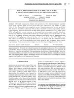
We use light physical activity as the outcome variable. PSID respondents are asked about
their physical activity habits in two questions. They first answer how often they do light
physical activity and then they report the time unit that allows to measure the frequency
of these activities (daily, weekly, monthly or annually). Based in these two questions we
construct a variable that indicates the number of times per week individuals do light physical
activity. It is an ordinal variable that assumes 44 different values, from 0 to 21. Its histogram
is presented in Figure 1. 15% of the observations in the sample report not doing physical
activity, while the remaining 85% do some positive number of light physical activity per week.
Two well-differentiated mass points -at values 0 and 7- can be identified. Also, more than
23% of the total number of observations lies in the interval (0,2] and other 23% are included
in the interval [2,7).
Figure 1: Histogram for the outcome variable: frequency of light physical activity (times per
week)
The two graphs in the left panel in Figure 2 show the average weekly frequency of light
physical activity by gender in 1999 and 2005 for treated and control individuals, pooling all
groups of states. We observe a downward trend in all groups for both genders. In particular,
for the groups of treated individuals the frequency of light physical activity goes down. This
simple Before-After estimator is telling us that HED policies have a negative impact on
11
the outcome of interest. However, this estimate is obviously biased given the fact that the
average of the outcome variable in the Treatment-non-Experimental group (Control 1) has
also a downward trend.
Exploring gender differences we can see that females in the Treatment-Experimental group
(Treated) present a larger drop in the frequency of light physical activity than that one

observed for males in the same group. This fact suggests the potential need for taking into
account gender differences when estimating the effect of HED policies.
Figure 2: Average frequency of light physical activity (times per week) by treatment/control
(left panel), by treatment groups (right panel) and by gender, in 1999 and 2005.
4.2
4.2
4.24.0
4.0
4.04.4
4.4
4.43.9
3.9
3.94.4
4.4
4.43.7
3.7
3.74.2
4.2
4.23.7
3.7
3.73
3
33.5
3.5
3.54
4
44.5
4.5
4.55
5

5Light physical activity (times per week)
Light physical activity (times per week)
Light physical activity (times per week)Treated
Treated
TreatedControl 1
Control 1
Control 1Control 2
Control 2
Control 2Control 3
Control 3
Control 399
99
9905
05
0599
99
9905
05
0599
99
9905
05
0599
99
9905
05
05Males
Males
Males4.5
4.5

4.53.6
3.6
3.64.5
4.5
4.53.9
3.9
3.94.3
4.3
4.33.7
3.7
3.74.4
4.4
4.43.6
3.6
3.63
3
33.5
3.5
3.54
4
44.5
4.5
4.55
5
5Light physical activity (times per week)
Light physical activity (times per week)
Light physical activity (times per week)Treated
Treated
TreatedControl 1
Control 1

Control 1Control 2
Control 2
Control 2Control 3
Control 3
Control 399
99
9905
05
0599
99
9905
05
0599
99
9905
05
0599
99
9905
05
05Females
Females
Females3.9
3.9
3.93.6
3.6
3.64.3
4.3
4.34.1
4.1

4.14.7
4.7
4.74.3
4.3
4.33
3
33.5
3.5
3.54
4
44.5
4.5
4.55
5
55.5
5.5
5.5Light physical activity (times per week)
Light physical activity (times per week)
Light physical activity (times per week) S4
S4
S4S5
S5
S5S6
S6
S699
99
9905
05
0599
99

9905
05
0599
99
9905
05
05Males
Males
Males3.9
3.9
3.93.6
3.6
3.64.8
4.8
4.83.7
3.7
3.74.7
4.7
4.73.2
3.2
3.23
3
33.5
3.5
3.54
4
44.5
4.5
4.55
5

55.5
5.5
5.5Light physical activity (times per week)
Light physical activity (times per week)
Light physical activity (times per week)S4
S4
S4S5
S5
S5S6
S6
S699
99
9905
05
0599
99
9905
05
0599
99
9905
05
05Females
Females
Females
Treated: individuals with children of elementary-school-age in experimental states. Control1: individuals with children
of elementary-school-age in non-experimental states. Control2: individuals without children of elementary-school-age in
experimental states. Control3: individuals without children of elementary-school-age in non-experimental states. The
type of policies corresponding to each group of states S are as follows. S4: topics unchanged and increase in the number
of enforcements; S5: implementation of topics and enforcements; S6: increase in the number of topics and enforcements.

As we discused above, the implementation and modification of HED policies between
1999 and 2005 was not homogenous across states. For this reason we may expect differences
12
in the temporal evolution of the outcome of interest for treated individuals across the three
groups of states previously defined as experimental states. The two graphs in the right panel
in Figure 2 show the average frequency of light physical activity for treated individuals by
gender and by group of experimental states. We see that for males residing in states belonging
to group S
5
the downward trend in the frequency of light physical activity is smaller than the
corresponding downward trend in groups S
4
and S
6
. Moreover, the reduction in the frequency
of light physical activity for males in group of states S
5
is lower than the fall in the frequency
of light physical activity for males in all three control groups. This moderate downward trend
for treated males in S
5
experimental states suggests the existence of a positive effect of HED
policies on the outcome variable.
In Table 3 we report descriptive statistics of the outcome variable, and other demographic
and socioeconomic characteristics in 1999 and 2005, for all individuals in the sample.
We find evidence of statistically significant differences in some observable characteris-
tics between 1999 and 2005, for individuals residing in Experimental and Non-Experimental
states. These differences may produce changes in the observed frequency of light physical
activity between 1999 and 2005, that are not a consequence of changes in HED programs. To
avoid a biased estimation of the effect of interest, we use a regression framework that allow

us to control for temporal differences in observable characteristics.
3.1 DDD estimation in a simple linear model
Table 4 presents the DDD estimate of the effect of changes in the HED policy on fathers’
behavior for a particular group of states, S
5
, in which both topics and enforcements where
implemented between 1999 and 2005 for the first time.
16
In this section we treat the outcome
variable, number of times per week individuals do light physical activity, as if it were a
continuous variable. With this assumption we cannot make valid quantitative interpretations
of the effect of the policy, but we can still make inference regarding the sign of the effect.
The top panel compares the change in the frequency of physical activity for fathers with
children of elementary-school-age residing in states S
5
to the change for fathers with children
16
In Table 12 we report results for a similar exercise on mothers.
13
Table 3: Descriptive statistics: all individuals in the sample.
Experimental states Non-Experimental states
1999 2005 Difference 1999 2005 Difference
(1) (2) (3) (4) (5) (6)
Frecuency of light physical 4.33 3.72 -0.61*** 4.39 3.74 -0.65***
activity (times per week) ( 2.95 ) ( 3.18 ) ( 3.14 ) ( 3.23 )
Proportion of Female 0.57 0.58 0.02 0.55 0.56 0.01
( 0.50 ) ( 0.49 ) ( 0.50 ) ( 0.50 )
Age 36.52 39.05 2.53*** 37.30 39.43 2.13***
( 8.09 ) ( 9.65 ) ( 8.00 ) ( 9.70 )
Years of Education 12.94 13.18 0.25 12.76 12.97 0.21*

completed ( 2.32 ) ( 2.23 ) ( 2.84 ) ( 2.61 )
Num. of Children 2.29 2.29 0.00 2.40 2.37 -0.04
( 1.23 ) ( 1.19 ) ( 1.28 ) ( 1.22 )
Num. of Children 0.55 0.41 -0.13*** 0.57 0.41 -0.16***
in elementary school ( 0.72 ) ( 0.66 ) ( 0.76 ) ( 0.66 )
Proportion of White 0.56 0.53 -0.03* 0.55 0.53 -0.02**
( 0.50 ) ( 0.50 ) ( 0.50 ) ( 0.50 )
Proportion of Married 0.76 0.75 -0.01 0.78 0.76 -0.02*
( 0.43 ) ( 0.43 ) ( 0.41 ) ( 0.43 )
Proportion of Unemployed 0.03 0.04 0.00 0.03 0.04 0.01**
( 0.18 ) ( 0.19 ) ( 0.18 ) ( 0.20 )
Proportion of Retired 0.00 0.01 0.00 0.01 0.01 0.01**
( 0.06 ) ( 0.08 ) ( 0.07 ) ( 0.10 )
Proportion of Disabled 0.02 0.03 0.01** 0.02 0.03 0.01***
( 0.13 ) ( 0.17 ) ( 0.14 ) ( 0.17 )
Labor income 13,917 19,092 5,174*** 15,072 20,054 4,981***
(per capita) ( 13,678 ) ( 21,944 ) ( 16,794 ) ( 31,862 )
Total income 16,375 25,711 9,335*** 18,124 23,738 5,613***
(per capita) ( 15,814 ) ( 124,101 ) ( 22,620 ) ( 35,656 )
Sample size 1,590 2,030 3,394 4,325
Stars in columns (3) and (6) show statistical significance of differences in proportion or distribution of the referred
variable, between years 1999 and 2005. We perform tests of difference in proportion for the dummy variables White,
Married, Unemployment, Retired, and Disabled. We perform tests of differences in distribution for the categorical
variables Frequency of light physical activity, Age, Education, Number of Children, and Number of Children in
elementary school, and for the continuous variables Labor income, and Total income. Significance levels: * = 10%;
** = 5%; *** = 1%.
14
of elementary-school-age in non-experimental states. Each cell contains the mean average
frequency of light physical activity for the group labeled on the axes, along with the standard
errors and the number of observations. The Before-After estimate (∆

T
E
) of the effect is
presented in the third column. There was a non-significant decrease in the frequency of light
physical activity for fathers with children of elementary-school-age in experimental states,
compared with a significant fall in the frequency of light physical activity for fathers with
children of the same age in other states. Thus, the diff-in-diff estimator (∆
T
E
−∆
T
NE
), reported
in the bottom part of the upper panel, is positive and significant; the relative frequency of
light physical activity of fathers with children of elementary-school-age has risen.
Table 4: DDD estimator for males in S
5
Before HED After HED Time
change change difference
A. Treatment individuals: with children in elementary school
Experimental states 4.255 4.138 -0.117 ∆
T
E
(0.270) (0.267) (0.380)
[150] [157]
Non-experimental states 4.867 3.200 -1.668*** ∆
T
NE
(0.357) (0.327) (0.484)
[59] [68]

Difference in difference 1.551**
(0.615)
B. Control Individuals: without children in elementary scchol
Experimental states 4.420 3.595 -0.825*** ∆
C
E
(0.188) (0.182) (0.262)
[229] [328]
Non-experimental states 4.206 4.043 -0.163 ∆
C
NE
(0.370) (0.268) (0.457)
[100] [150]
Difference in difference -0.662
(0.527)
DDD = (∆
T
E
− ∆
T
NE
) − (∆
C
E
− ∆
C
NE
) 2.213***
(0.810)
Cells contain mean frequency of light physical activity for the group identified. Standard errors are given in paren-

theses, and sample sizes in brackets. The non-experimental states are groups of states S1, S2 and S3. Significance
levels: * = 10%; ** = 5%; *** = 1%.
If there were a different shock common to the experimental states that affected fathers’
frequency of physical activity, the previous estimator does not identify the spillover effects
of the implementation of HED policies. In the middle panel of Table 4 we perform the
same exercise for the groups of fathers with children above and bellow elementary-school-
15
age. For those groups we find a fall in the relative frequency of light physical activity in the
experimental states, relative to the other states. Although not significant, this suggests that
it may be important to control for state-specific shocks in estimating the impact of HED
policies.
Taking the difference between the two panels of Table 4, we obtain a significant increase
in the relative frequency of physical activity for fathers of children in elementary-school-age
in the states that implemented HED requirements, compared to the change in the relative
frequency of physical activity in non-experimental states. This statistically significant DDD
estimate provides some evidence on the existence of spillovers of HED on fathers’ physical
activity. However, its quantitative interpretation is problematic since the support of the
outcome variable is not the real line. We discuss in the next Section how the DDD design
can be expressed within a regression framework in which we can explicitly model the discrete
support of the outcome variable as well as we can control for observed characteristics.
3.2 Empirical model
Our outcome variable, the number of times per week individuals do light physical activity,
is an ordinal variable for which the value of the outcome reflects relevant information. We
may say that a higher value of the outcome variable is better than a lower value, since
doing a higher number of light physical activity per weeks is better (in terms of health
status benefits) than doing less light physical activity. Ideally, we would like to use this
information provided by an ordinal variable, by estimating the effect of interest in an ordered
response model. Unfortunately, in PSID database there is no information on how much time
individuals spend in doing physical activity. That is, we know how many times per week
they do physical activity but we do not know for how long they do physical activity in each

reported session. In our database, an individual that reports doing light physical activity
three times per week is not necessarily doing more light physical activity than an individual
who reports one session per week.
Given this limitation, we use as the outcome variable a binary variable that reflects
whether an individual does any positive number of light physical activity per week.
16
In what follows, the outcome variable is:
y
i
=





0 if i does not do light physical activity
1 if i does light physical activity
The latent variable version of the model with three types of treatment has the following
form:
y
∗
itj
= β
0
+ β
1
τ
t
+ β
2

elem
i
+
6

k=1
β
3,k
S
k
+
β
4
(elem
i
× τ
t
) +
6

k=1
β
5,k
(S
k
× τ
t
) +
6


k=1
β
6,k
(S
k
× elem
i
)+
6

k=4
β
7,k
(S
k
× elem
i
× τ
t
) + β
8
X
itj
+ u
itj
,
(1)
where i = 1 N indexes individuals, t = 0, 1 indexes time (0=before policy, 1999; 1=after
policy, 2005), j = 1 38 indexes states and k = 1, , 6 indexes state groups; τ
t

is a dummy
variable, equal one in 2005; S
k
is a dummy equal one if the individual resides in the state j
that belongs to group k; elem
i
is a dummy equal one if individual i has children of elementary-
school-age (children aged between 6 and 10 years old); and X
itj
is a set of observable individual
characteristics including age, race, gender, marital status, number of children, children of
high-school-age, education level, employment status, total family income level and state of
residence.
This specification controls for time trend in the dependent variable (β
1
), for time-invariant
characteristics of the treatment group (β
2
), and for time-invariant characteristics of the dif-
ferent groups of states ({β
3,k
}
6
k=1
). The second-level interactions control for changes over
time for the treatment group nationwide (β
4
), changes over time in each group of states
({β
5,k

}
6
k=1
), and time-invariant characteristics of the treatment group in each group of states
({β
6,k
}
6
k=1
). The third-level interactions ({β
7,k
}
6
k=4
) capture variation in the relative proba-
bility of physical activity specific to the treatments (relative to controls) in the experimental
states with respect to the non-experimental states in the year after the HED requirements
17
changed. These are the DDD estimates and they capture the effects of the different policies.
Given the existence of different time trends on the frequency of light physical activity
between females and males observed in Figure 2, the model we estimate also interacts the
policies with a dummy variable that takes value 1 if the individual is female. The model with
interactions by gender has the following form:
y
∗
itj
= β
0
+ β
1

τ
t
+ β
2
elem
i
+
6

k=1
β
3,k
S
k
+ β
4
female
i
+ β
5
(τ
t
× female
i
) + β
6
(elem
i
× female
i

)+
6

k=1
β
7,k
(S
k
× female
i
) + β
8
(elem
i
× τ
t
) + β
9
(elem
i
× τ
t
× female
i
) +
6

k=1
β
10,k

(S
k
× τ
t
)+
6

k=1
β
11,k
(S
k
× τ
t
× female
i
) +
6

k=1
β
12,k
(S
k
× elem
i
) +
6

k=1

β
13,k
(S
k
× elem
i
× female
i
)+
6

k=4
β
14,k
(S
k
× elem
i
× τ
t
) +
6

k=4
β
15,k
(S
k
× elem
i

× τ
t
× female
i
) + β
16
X
itj
+ u
itj
.
(2)
The DDD estimates in this model are β
14,k
for males, and β
14,k
+ β
15,k
for females. If
the coefficient β
15,k
is significantly different from zero, then there is evidence of a differential
impact of HED policies among fathers and mothers. We estimate the parameters of interest
by Maximum-Likelihood and we compute standard errors corrected for cluster at family level.
A report of the estimated coefficients can be found in Table 13 in the Appendix.
4 IATE estimates
In this Section we report the estimates of the Indirect Average Treatment Effect (IATE).
The IATE is computed as the average value of the indirect treatment effect across treated
individuals.
Let ˆπ

k
= (β
0
, β
1
, β
2
, {β
3,k
}
6
k=1
, β
4
, {β
5,k
}
6
k=1
, {β
6,k
}
6
k=1
, β
8
) be the vector of estimated pa-
rameters without including the parameters that measure policy effects ({β
7,k
}

6
k=4
). Similarly,
let Z
itj
be the vector of variables for the individual i at time t = 2005 residing in state j
without including the third level interaction variable S
k
× elem
i
× τ
t
.
The IATE across treated individuals in the group of states S
k
is computed using the
following expression:
18

i: elem=1&S
k
=1
[Φ(ˆπ
k
Z
kit
+ β
7,k
(S
k

× elem
i
× τ
t
)) − Φ(ˆπ
k
Z
kit
)]/N
kt
, (3)
where Φ stands for the normal distribution function, and N
kt
is the number of treated indi-
viduals in the group of states S
k
at time t = 2005.
We report in Table 5 the IATE for the three different types of treatment.
Table 5: IATE across treated individuals.
Male Female
OLS Probit # obs OLS Probit # obs
S4: Topics unchanged & -0.016 -0.031 85 -0.049 -0.041 124
Enforcements increase (0.071) (0.079) (0.064) (0.071)
S5: Topics introduced & 0.102* 0.142* 157 -0.011 -0.018 215
Enforcements introduced (0.057) (0.083) (0.047) (0.055)
S6: Topics increase & 0.070 -0.018 29 0.0003 0.014 47
Enforcements increase (0.091) (0.140) (0.091) (0.1759)
Cluster set at family level. Bootstrap standard errors with 1000 replications. The regression
includes the following covariates: age, race, gender, marital status, number of children, children
of high school-age, education level, employment status, total family income level, and state of

residence. Significance levels: * = 10%; ** = 5%; *** = 1%.
We find evidence of a positive effect of HED education at elementary school on parents’
probability of engaging in light physical activity. Requiring topics and enforcements for the
first time (S
5
group of states) raises fathers’ probability of doing physical activity. Looking
at the results of the probit model we can see that the probability of doing physical activity
for a father affected by this policy is 14.2 percentage points higher than a comparable father
not affected by the policy. The positive and statistically significant effect on fathers is also
obtained by using a linear probability model. The effect on mothers’ probability of physical
activity is never statistically significant, but interestingly the signs are the opposite of those
found for fathers.
The estimated effects are not statistically significant for males and females residing in
groups of states S
4
and S
5
. These results suggest that once the HED has been implemented,
changes in its implementation does not have an additional indirect effect.
We conclude that there are positive spillovers of the implementation of HED for the first
time on fathers’ probability of doing physical activity, while for mothers we do not find a
19
statistically significant effect of these reforms.
4.1 Plausible explanations for our results
We can think of two channels explaining our results. When children start receiving HED
at school they parents are confronted with two new sets of factors that might potentially
affect their health-related behavior. First, parents may optimally react to HED in schools
by complementing this education with the incorporation of healthy lifestyles into their own
daily activities. We refer to this potential channel as “role modeling”. On the other hand,
there is the effect of the arrival of new information that the child receives at the school. In

particular, parents are faced up to the knowledge that the child brings to the household from
the health education curricula given at the school, and they may adjust their health behaviors
in response to it. We refer to this potential channel as “information sharing”.
In what follows we provide evidence on the existence of both channels.
4.1.1 Role models
Parents may do more physical exercise in response to the knowledge children acquired via
HED, not because they weren’t aware of the benefits of exercising but because they want to
complement the instruction received by the child so as to form the desired healthy lifestyle
in the child.
The estimates from the model interacting the policies with a dummy variable for gender
allow us to obtain some insights on the operation of the “role model” channel. Parents usually
spend more time with their children doing gendered activities. Figure 3 in the Appendix shows
some evidence in this respect with data coming from the American Time Use Survey (ATUS).
Women spend roughly twice as much time in childcare as do men, a pattern which holds true
for all subgroups and for almost all types of childcare, except for “Recreational” childcare.
This type of childcare activities includes playing games with children, playing outdoors with
children, attending a child’s sporting event or dance recital, going to the zoo with children,
taking walks with children, etc. In the case of “Recreational” childcare, mothers allocate
relatively less of their time with children when compared with the time allocation into types
of childcare activities that fathers do. Thus, this is evidence on the fact that fathers are more
20
likely to do stereotypically male activities with their children, among which physical activity
is included. Accordingly, the impact of HED reforms on physical activity is also expected to
appear for fathers rather than for mother.
4.1.2 Information sharing between children and parents
Individuals with lower stock of information are expected to be more affected by HED changes.
We explore the existence of the information sharing channel by analyzing the differential
impact of HED reforms on individuals with low and high education levels and with low and
high income levels. Since lower level of education and socioeconomic status are related with
less knowledge about health (Tinsley, 2003), we expect to obtain a higher effect of HED

reforms on individuals with lower level of education and income.
Exploiting the non linearity of the model specified we estimate IATE evaluated at partic-
ular values of the covariates of interest. We report the results in Table 6 for treated fathers
residing in states that belong to group S
5
. According to these results, the policy has a higher
effect on low educated males relative to high educated males, on non-white males relative
to white males, and on males that have a lower income than those having a higher income.
The policy rises in 4 percentage points more the probability of being physically active of low
educated males relative to high educated males, whereas the increment was 3.8 percentage
points higher for non-white males relative to white males.
Table 6: Differences in IATE estimates evaluated at particular values of the covariates.
Income IATE Education IATE Race IATE
Low 0.145* Low 0.158* No White 0.164*
(20th percentile) (0.085) (0.090) (0.093)
High 0.140* High 0.117 White 0.126
(80th percentile) (0.083) (0.072) (0.077)
Difference 0.004* 0.041** 0.038**
(0.002) (0.020) (0.018)
Cluster set at family level. Bootstrap standard errors with 1000 replications. We find no differences
for males in family size, labor force participation, and marital status. There exist no differences
for females in all the dimensions analyzed. Significance levels: * = 10%; ** = 5%; *** = 1%.
21
5 Conclusion
We find evidence on the existence of positive spillovers of HED imparted in elementary schools
on parents’ probability of engaging in light physical activity. However, our results suggest
that fathers and not mothers are those affected by the HED reforms. We also analyze the
differential impact of HED reforms on fathers and mothers as a way to explore the nature of
the channels driving the spillovers.
We argue that the existence of a “role model” channel can explain the differential impact

on fathers and mothers. The idea is based on the fact that there are different role models
that mothers and fathers play for their children. Parents usually spend more time with their
children doing gendered activities. Since physical activity can be included into the group of
the typically male-activities, the effect of the promotion of the advantages of doing physical
activity is more likely to appear for fathers rather than for mothers. We also explore the
existence of a second channel driving our results -the “information sharing” channel- by
analyzing the differential impact of HED reforms on individuals with low and high education
levels, and we obtained the expected higher effect on less educated individuals and individuals
with a lower socioeconomic status.
Our results also highlight the importance of clearly distinguishing the existence of several
dimensions in the implementation of a policy. In our case, considering the two dimensions in
the HED reforms -changes in topics and enforcements- as well as the distinction between im-
plementing requirements for the first time relative to reforms in already existing requirements
is important for the policy evaluation. Our main result shows the existence of spillovers only
in the case when both policy dimensions are simultaneously implemented for the first time.
The existence of spillovers of HED on parental lifestyles indicates that the interaction
between children and parents play a role in the formation of healthy lifestyles inside the
household. Therefore, taking into account these spillovers is important in the cost-benefit
analysis of introducing health education at schools. In addition, the conclusion that im-
plementing reforms in topics is not enough to obtain spillovers at the family level helps to
properly design policy interventions aiming to increase the acquisition of healthy lifestyles in
a given community.
22
References
Angelucci, M. and G. D. Giorgi (2009): “Indirect Effects of an Aid Program: How
Do Cash Transfers Affect Ineligibles’ Consumption?” American Economic Review, 99,
486–508.
Bhattacharya, J., J. Currie, and S. J. Haider (2006): “Breakfast of Champions?:
The School Breakfast Program and the Nutrition of Children and Families,” J. Human
Resources, XLI, 445–466.

Cawley, J., C. Meyerhoefer, and D. Newhouse (2007): “The impact of state physical
education requirements on youth physical activity and overweight,” Health Economics, 16,
1287–1301.
Clark, A. E. and F. Etile (2006): “Don’t give up on me baby: Spousal correlation in
smoking behaviour,” Journal of Health Economics, 25(5), 958–978.
Currie, J. (2009): “Healthy, Wealthy, and Wise: Socioeconomic Status, Poor Health in
Childhood, and Human Capital Development,” Journal of Economic Literature, 47, 87–
122.
Gruber, J. (1994): “The Incidence of Mandated Maternity Benefits,” American Economic
Review, 84, 622–41.
Guryan, J., E. Hurst, and M. Kearney (2008): “Parental education and parental time
with children,” Journal of Economic Perspectives, 22, 23–46.
Jacoby, H. G. (2002): “Is There an Intrahousehold ”Flypaper Effect”? Evidence From a
School Feeding Programme,” Economic Journal, 112, 196–221.
Kann, L., N. D. Brener, and D. Allensworth (2001): “Health education: results
from the School Health Policies and Programs Study 2000,” Journal of School Health, 71,
266–278.
Kann, L., S. Telljohann, and S. Wooley (2007): “Health Education: Results from the
School Health Policies and Programs Study 2006,” Journal of School Health, 77, 408–434.
23
Kenkel, D. S. (2000): “Prevention,” Handbook of Health Economics, 1, 1675–1720.
Lalive, R. and A. Cattaneo (2006): “Social Interactions and Schooling Decisions,” IZA
Discussion Papers 2250, Institute for the Study of Labor (IZA).
McGeary, K. A. (2009): “The Impact of State-Level Nutrition-Education Program Funding
on BMI: Evidence from the Behavioral Risk Factor Surveillance System,” NBER Working
Papers 15001, National Bureau of Economic Research, Inc.
Miguel, E. and M. Kremer (2004): “Worms: Identifying Impacts on Education and
Health in the Presence of Treatment Externalities,” Econometrica, 72, 159–217.
Shi, X. (2008): “Does an intra-household flypaper effect exist? Evidence from the educa-
tional fee reduction reform in rural China,” mimeo.

Tinsley, B. J. (2003): How children learn to be healthy, Cambridge University Press.
WHO (1999): “Improving health through schools: national and international strategies,”
http : //www.who.int/school
y
outh
h
ealth/media/en/94.pdf.
——— (2003): “Health and Development Through Physical Activity and Sport,” http :
//whqlibdoc.who.int/hq/2003/W HO NM H NPH P AH 03.2.pdf.
Wyatt, T. and J. Novak (2000): “Collaborative partnerships: a critical element in school
health programs,” Family & Community Health, 23, 1.
24
Appendix
Table 7: States That Require Elementary Schools to Teach Health Topics, by Topic and Year
2000 2006
State topic 1 topic 2 topic 3 topic 4 topic 5 topic 1 topic 2 topic 3 topic 4 topic 5
Alabama yes yes yes yes yes yes yes yes yes yes
Alaska no no no no no no no no no no
Arizona no no no no no no no no no no
Arkansas no no no no no no no yes yes no
California yes yes yes yes yes yes yes yes no yes
Colorado no no no no no no no no no no
Connecticut yes yes yes yes yes yes yes yes yes yes
Delaware yes yes yes yes yes yes yes yes yes yes
District of Columbia yes yes yes yes yes yes yes yes yes yes
Florida no no no no no yes yes yes no no
Georgia yes yes yes no yes yes yes yes yes yes
Hawaii no no no yes no yes yes yes yes yes
Idaho no no no no no yes yes yes yes yes
Illinois yes yes yes yes yes yes yes yes yes yes

Indiana yes yes yes yes yes yes yes yes no yes
Iowa yes yes yes yes yes yes no yes no yes
Kansas no no no no no no no no no no
Kentucky yes yes yes yes yes yes yes yes yes yes
Louisiana yes yes yes yes yes yes yes yes no yes
Maine yes yes yes no yes yes yes yes yes yes
Maryland yes yes yes yes yes yes yes yes yes yes
Massachusetts yes yes yes yes yes yes yes yes yes yes
Michigan yes yes yes no yes yes yes yes no yes
Minnesota yes no yes yes yes no no no no no
Mississippi yes yes yes yes yes no no no yes no
Missouri yes yes yes yes yes yes no no no yes
Montana yes yes yes yes yes yes yes yes yes yes
Nebraska yes no no no yes yes no yes yes yes
Nevada yes yes yes yes yes yes no yes yes yes
New Hampshire yes yes yes yes no yes no no no no
New Jersey yes yes yes yes yes yes yes yes no yes
New Mexico no no no no no yes yes yes yes yes
New York yes yes yes yes yes yes yes yes yes yes
North Carolina yes yes yes yes yes yes yes yes yes yes
North Dakota yes no no no yes yes no no yes yes
Ohio yes no yes yes yes no no no no no
Oklahoma yes yes yes yes yes no no no no no
Oregon yes yes yes yes yes yes no no no yes
Pennsylvania yes no no no yes yes yes yes yes yes
Rhode Island yes yes yes yes yes yes yes yes yes yes
South Carolina yes yes yes yes yes yes yes yes yes yes
South Dakota no no no no no no no no no no
Tennessee yes yes yes yes yes yes yes yes yes yes
Texas no no no no no yes yes yes yes yes

Utah yes yes yes yes yes yes yes yes yes yes
Vermont yes yes yes no yes yes yes yes yes yes
Virginia yes yes yes yes yes yes yes yes yes yes
Washington yes no yes yes yes yes yes yes yes yes
West Virginia yes yes yes yes yes yes yes yes yes yes
Wisconsin yes yes no no yes no no no no no
Wyoming no no no no no no yes no no no
Source: School Health Policies and Programs Study (SHPPS).
Topic 1:Alcohol or other drug-use prevention; Topic 2: Emotional and mental health; Topic 3: Nutrition and dietary behavior;
Topic 4: Physical activity and fitness; Topic 5: Tabacco-use prevention.
25