Impact Of Wildlife Recreation On Farmland Values pot
Bạn đang xem bản rút gọn của tài liệu. Xem và tải ngay bản đầy đủ của tài liệu tại đây (357.65 KB, 22 trang )
1
THE IMPACT OF WILDLIFE RECREATION ON FARMLAND VALUES
Jason Henderson and Sean Moore*
Center for the Study of Rural America
December 11, 2005
RWP 05-10
Abstract: Wildlife recreation – hunting, fishing, and wildlife watching – appears to be an
increasingly important past time for many Americans as people continue to increase their
spending on wildlife recreation. Land lease and ownership expenditures by wildlife recreation
participants are rising and appear to be capitalized into farmland values. This paper analyzes the
impact of hunting lease rates on farmland values in Texas. The results indicate that counties with
higher wildlife recreation income streams have higher land values.
Keywords: farmland values, wildlife recreation
JEL Classification: Q15
*Authors are Senior Economist and Research Associate, Center for the Study of Rural America,
Federal Reserve Bank of Kansas City, 925 Grand Boulevard, Kansas City, MO 64198, USA. The
authors benefited from the comments of participants at the Agricultural and Rural Finance
Markets in Transition Conference. The views expressed are those of the authors and do not
reflect the views of the Federal Reserve Bank of Kansas City or the Federal Reserve System.
Henderson email:
Moore email:
2
1. Introduction
Wildlife recreation – hunting, fishing, and wildlife watching – has garnered increasing
attention as an engine of economic development in rural communities. The expansion and
success of rural outfitter businesses, such as Cabella’s and Bass Pro Shop, are clear examples of
the economic possibilities of wildlife recreation activity. Other examples are the emerging
businesses engaged in hunting and trapping industries. From 1998 to 2003, the hunting and
trapping industry grew 25 percent in the number of firms and employment and 50 percent in
terms of payroll.
1
More recently, wildlife recreation has emerged as an increasing influence affecting U.S.
farmland as farmers are capturing additional income streams from wildlife recreation. In 2002,
more than 2800 farms averaged $7,217 dollars from recreation services, where recreation service
income was characterized as hunting and fishing (NASS). Surveys of land values indicate that
recreation activity is fueling a surge in land values. In Texas, 68 percent of land market
professionals indicated that hunting and fishing was a dominant motive for land buyers in 2003
(Gilliard, Robertson, and Cover). In a survey of agricultural bankers in the Kansas City Federal
Reserve District, 57 percent reported that recreation demand was a contributing factor in
farmland value gains in December 2004, up from 44 percent in December 2002 (Center for the
Study of Rural America).
2
Wildlife recreation creates additional demand for land and opens up opportunities for
additional revenue streams. Since farmland values are capitalized values of expected earnings,
increased revenues from wildlife recreation should fuel farmland values gains. Research has
1
Calculations based on 1998 and 2003 County Business Patterns data for the hunting and trapping industry (NAICS
code 1142).
2
The Kansas City Federal Reserve District covers that states of Nebraska, Kansas, Oklahoma, Colorado, Wyoming,
northern New Mexico, and western Missouri.
3
focused on the impact of recreation and scenic amenities on land values. Wildlife recreation is
unique from other recreation activities because it does not necessarily lead to the conversion of
farmland to non-farm activities. The land value impacts of wildlife recreation might be different
from scenic amenities because wildlife recreation is a public good that may produce private
benefits. Similar to scenic amenities, wildlife is a public good. By controlling hunting and
fishing access to private land, land owners control access to wildlife and may be able to capture a
private benefit. For example, some farmers lease their land for hunting and receive an additional,
complementary farm income stream.
3
Given the apparent rise in recreational demand for farmland, this paper analyzes the
impacts of wildlife recreation on farmland values. After reviewing previous literature, a hedonic
price model of farmland values is used to identify the impact of hunting lease rates and
recreational income on farmland values in Texas. The results indicate that farmland values in
Texas are higher in counties with higher hunting lease rates and greater recreational income for
farmers, ceteris paribus.
2. Literature Review
Farmland is a resource used in a variety of activities, including wildlife recreation, and its
value is derived from the capitalized value of its expected future returns. Agricultural income,
including farm program payments, is the primary revenue stream for farmland. A large number
of studies have analyzed the capitalization of agricultural income streams into farmland values
(Barnard et al. 1997; Burt 1986; Chavas and Shumway 1982; Castle and Hoch 1982;
Featherstone and Baker, 1987; Herriges et al, 1992; Just and Miranowski, 1993; Moss, 1997;
3
The presence of wildlife can also present costs to farmers. For example, high densities of wildlife can lead to
severe crop damage or increased probability of automobile accidents.
4
Miranowski and Hammes, 1984; Phipps, 1984). Some of these studies have used time-series
data, while others have used cross-sectional data.
Another group of studies has focused on the impacts of urbanization on farmland values
(Chicoine, 1981; Clonts, 1970; Dunford et al, 1985; Folland and Hough, 1991; Reynolds and
Tower, 1978; Shi et al, 1997; Shonkwiler and Reynolds, 1986). The primary hypothesis in these
studies is that the potential for future urban expansion and the conversion of farmland into
residential or commercial use is being capitalized into farmland values. In general, these studies
find that the potential for urban development is being capitalized into farmland values with
regions closer to large and growing urban centers experiencing higher land values. Most of these
studies focus on the spatial variation of farmland values.
Recent literature has also analyzed the impacts of scenic or wildlife amenities on land
prices. Research has found higher land prices in places containing or in close proximity to scenic
amenities. Irwin (2002) and Irwin and Bocksteael (2001) found that residential prices are higher
in areas with more open space. Irwin and Bockstael (2004) indicate that land near preserved or
unprotected open space has greater probability to be developed than land in closer proximity to
commercial or neighborhood development.
Research has also found that places with greater wildlife amenities have higher land
values. Bastian (2002) found that wildlife amenities were associated with higher agricultural land
values in Wyoming. Land with scenic views, elk habitat, and sport fishery had higher land
values.
4
Pope, Adams, and Thomas (1984) and Pope (1985) using data from a survey of Texas
hunters found that land values in Texas were higher in regions with greater deer harvest
densities.
4
Research has also analyzed the impact of the recreation industry on farmland values. Barnard, et. al (1997) found
that farmland values were higher in counties with higher per capita wages in the recreation industry - resorts and
attractions.
5
Another body of research has focused on the influence of land attributes on wildlife
recreation leases. Livengood (1983) analyzed the value of hunting lease and the marginal
willingness to pay for hunting white-tailed deer in Texas in 1978 and 1979. Pope and Stoll
(1985) also analyzed the hunting lease prices for white-tailed deer in Texas and found that the
location and size of the hunting parcel and the diversity of hunting game influenced hunting
leases. Baen (1997) analyzed Texas hunting leases and developed a hunting lease index based on
the deer densities, trophy quality deer, and metro proximity of rural lands. Shrestha and
Alavalapati (2004) analyzed the impact of various ranchland attributes on Florida hunting leases
and find that vegetation cover has a positive impact on hunting revenues.
Despite the research analyzing the impact of land attributes on hunting leases, research
analyzing the capitalization of wildlife recreation income streams into farmland values is limited.
Pope, Adams, and Thomas (1984) and Pope (1985) combined recreation income with other
agricultural income in their models. As a result, these studies were unable to identify the impacts
of recreation income from other agricultural income streams.
3. Texas Wildlife Recreation Income
The primary challenge in analyzing the economic impact of wildlife recreation on
farmland values is to obtain secondary measures of income from wildlife recreation. However,
Baen (1997) provides average per acre hunting lease rates for 115 Texas counties for 1996.
These averages were obtained from the 1996 Texas Farm and Ranch Hunting Survey by the
office of the Texas Comptroller and Public Accounts. Landowners were randomly selected in
each of the Texas counties from landowner tax rolls. The response rate was 16 percent and
6
responses covered 142 out of the 254 counties.
5
Figure 1A shows the hunting lease rates by
county for a 12 month access lease.
6
Over 80 percent of the landowners with lease arrangements
reported leases covering deer hunting. As a result, the geographic coverage of the hunting lease
rates in Figure 1A appears to overlap with the deer densities in Texas as shown in Figure 1B.
Capitalizing hunting income at a three percent rate, Baen indicates that the hunting value
averaged 25 percent of the market value of farmland in the corresponding counties. In some
counties, the hunting value accounted for more than two-thirds of the market value of farmland.
While Baen’s data series limits analysis to the state of Texas, Texas appears to be a
viable state to analyze the impact of wildlife recreation on farmland values. Baen reports that 98
percent of Texas land was privately owned. Pope and Baen indicate that the market for access to
wildlife was developed in the 1980s and 1990s. The U.S. Fish and Wildlife Service (1996)
reports that over 80 percent of the big game hunters hunted only on private land. Moreover, in
1996 and 2001, Texas ranked first in hunting expenditures with $1.5 billion dollars spent on
hunting (Table 1). Texas also ranked first with 1.2 million hunting participants. According to the
2002 Census of Agriculture, Texas ranked first in the number of farms receiving income from
recreation services (8,230) and in the total value of income they received ($77.6 million).
4. Empirical Model
Given that farmland values are derived from the capitalization of the expected future
income streams derived from multiple and sometimes competing uses, the hunting lease data is
used in a hedonic price model to analyze their impact on Texas farmland values. In hedonic
5
See Baen for more detail on the survey design, sample, and response rates.
6
Hunting leases can be highly variable in their design ranging from annual, season, day, to gun leases. See Baen
(1987) and Pope (1985) for a description of typical lease arrangements in Texas.
7
models, prices of heterogeneous goods are determined by the goods’ characteristics. Hedonic
price models have been used extensively to impute the value of agricultural land attributes in
farmland prices (Miranowski and Hammes 1984; Palmquist and Danielson 1989; Herriges et al.
1992; Roka and Palmquist 1997). Hedonic models have also been used to analyze residential
property values (Irwin 2002).
The hedonic price model is specified as:
P= f(A, U, S, H) (1)
where the dependent variable P is the county level per acre farmland values in Texas counties in
2002. The data was obtained from the 2002 Census of Agriculture at
A is a vector of agricultural attributes, U is a vector of non-
agricultural attributes, S is a vector of scenic, environmental, or recreation attributes, and H is the
hunting lease rate variable. Table 2 provides descriptive statistics on the data.
4.1. Control Variables
A series of variables are used to control for the non-recreational attributes influencing
farmland values. Three variables control for the impacts of the county’s agricultural economy on
farmland values. The average annual county level per acre crop receipts from 1997 to 2000,
CROP, is included to measure the economic returns to crop farming. The average county level
per acre livestock receipts from 1997 to 2002, LSTK, is included to measure the economic return
to livestock farming. Counties with larger crop or livestock returns are assumed to have higher
capitalized farmland values.
Farm incomes have also been supported by government payments. GOV, the average
annual per acre value of government payments received in the county between 1998 and 2000, is
used to measure the farm income stream derived from federal subsidies. Counties with higher
8
levels of government payments are expected to have higher demand for farmland and higher land
values. A positive relationship between GOV and farmland values is expected.
Multiple variables are used to control for the urban impacts on farmland values. A
dummy variable, METRO, identifies counties that are classified as a metro area. Another dummy
variable, ADJACENT, identifies non-metropolitan counties are adjacent to metro areas. Both
variables are include to measure the impacts of urban sprawl on farmland demand as
metropolitan areas grow in size and spread into neighboring non-metropolitan counties. The
population density of the county in 1990, POPDEN, and the average annual population growth
from 1990 to 2000, POPGROW, are used to measure the impacts of a large and growth
population on the demand for farmland for residential use in larger non-metropolitan counties. In
fact, much of the recent economic growth has been emerging from newly classified micropolitan
counties, non-metro counties with a city between 10,000 and 50,000 in population (Henderson
and Weiler). Farmland values are hypothesized to be positively related to METRO, ADJACENT,
POPDEN, and POPGROW because of higher demand for land near large and growing
populations with more abundant urban amenities.
Natural amenity data are used to control for the impact of scenic and environmental
amenities on farmland values. McGranahan (1999) describes the development of the natural
amenity index based on various weather and geographic variables. Due to the expected high
correlation between crop productivity and weather conditions, we only include a geographic
index based on typography and water surface area.
7
Standardized land surface form typography
codes and water surface area data for all U.S. counties are obtained from USDA Measuring
Rurality Briefing Room. The standardized data are then summed and indexed to 100.
7
Additional analysis used McGranahan’s natural amenity index and found a high correlation between this index and
weather measures. Models including these measures found the amenity and weather indexes to be highly significant,
but led to insignificant results for crop receipts per acre (CROP) variable.
9
4.2. Wildlife recreation variables
The initial variable used to measure recreation income is the average hunting lease rate in
1996 provided by Baen (1987). The lease rate is based on a twelve month annual access. The
hunting lease variable, HUNTING, is expected to be positively related to farm land values.
One drawback of the hunting lease variable is that it is derived from a relatively small
sample. A total of 414 surveys were obtained in the 1996 survey for an average of roughly three
per county.
8
To check for the robustness of the results, alternative specifications are estimated
that replace the hunting lease variable with other proxy measures of recreation income. Given the
availability of total county recreation service income and farms receiving recreation service
income in the 2002 Census of Agriculture, the average recreation service income per farm was
calculated. However, a preferred method would identify income on a per acre basis, because
farm sizes can be highly variable. Thus, an alternative measure, RECACRE, approximates the
average income per acre by dividing average recreation service income per farm by the average
farm size in the county. RECACRE is expected to be positively related to farmland values.
For a further check for reboustness, we included the number of deer per acre for Texas
counties. The deer density measure, DEERDEN, will not analyze the capitalization of wildlife
recreation income, but the capitalization of wildlife attributes into Texas farmland values.
DEERDEN is expected to be positively related to Texas farmland values.
While average lease rates may influence farmland values, land values may also be
influenced by the total size of the wildlife recreation market. For example, a hunting lease rate
may be high, but if a single hunting lease transaction occurs in the county, it would have limited
impacts on farmland values. The size of the wildlife recreation market is measured by the
8
According to the 2002 Census, 8230 farms received income from recreation services. Assuming no change in the
number of farms receiving recreation services income from 1996 to 2002, means that the lease rates would be
derived from approximately 5 percent of the population.
10
number of farms receiving income from recreation services (hunting, fishing, etc.) in 2002 as
reported in the Census of Agriculture. Counties with larger recreation service markets are
expected to have greater impacts on farmland values.
9
5. Empirical Results
Regression results for the estimated farmland price models are presented in Table 4. The
model was applied to 114 Texas counties for which hunting lease rates were reported in Baen
(1997).
10
The initial model included only the hunting lease rate. To check for robustness of
results, alternative specifications placed the hunting lease rate with recreation income measures
and wildlife recreation attributes as described previously. Both linear and log-linear forms of the
model were estimated, and the log-linear form is used because it minimizes Akaike’s
Information Criterion (AIC).
11
The model appears to have good fit according to the adjusted R
2
measures. The potential for spatial autocorrelation was addressed following Rappaport (2003).
12
In Model 1, the control variables are statistically significant at the 0.10 level with the
hypothesized sign, except GOV. The insignificance of GOV may due to collinearity with CROPS
9
The total county farm recreation service income in 2002 was also used to measure the size of the wildlife
recreation market in the county. The number of farms receiving recreation income (FARMS) was used because it
would provide a better approximation of the number of recreation lease transactions in the county. Moreover,
Akaike’s Information Criterion (AIC) was minimized when the FARMS measure was used.
10
Disclosure problems associated with the government payments variable limited the observations to 114 counties.
11
Theory provides little guidance in the choice of the model’s functional form. The common approach is to select
the functional form that minimizes goodness of fit criterion for the model (Irwin, 2002).
12
Rappaport (2003) used a generalization of the Huber-White heteroskedastic-consistent estimator to report
standard errors to account for spatial autocorrelation among disturbance terms. The following declining weighting
function for estimating the covariance between disturbances is imposed on counties with a Euclidean distance less
than 100 kilometers between county centers, where s
ij
is the estimate of
ij
σ
and u
i
is the regression residual.
S
i,j
= g(distance
i,j
) u
i
u
j
where
g(distance
i,j
)
= 1 : distance
i,j
=0
=: 0 <distance
i,j
100 km
= 0 : distance
i,j
>100 km
≤
2
ji,
100
distance
1
⎟
⎟
⎠
⎞
⎜
⎜
⎝
⎛
−
S
i,j
= g(distance
i,j
) u
i
u
j
where
g(distance
i,j
)
= 1 : distance
i,j
=0
=: 0 <distance
i,j
100 km
= 0 : distance
i,j
>100 km
≤
2
ji,
100
distance
1
⎟
⎟
⎠
⎞
⎜
⎜
⎝
⎛
−
11
as the variance inflation factors for GOV and CROPS are greater than two (Judge et al 1985).
13
The high degree of collinearity is not surprising given that government payments are primarily
received by crop producers and are based on productivity of the land.
Variables controlling for the agricultural attributes of the county are significant with the
hypothesized signs and consistent with other research results. Counties that have higher crop and
livestock cash receipts per acre had higher land values. Farmland that offers a higher expected
return from agricultural production has a higher capitalized value, ceteris paribus.
Variables controlling for the impacts of urban attributes of the county are significant with
the hypothesized sign. Demand for land in urban use and thus land values are higher in places
with larger concentrations of people. Farmland values are higher in counties with higher
population density. Moreover, farmland in metro counties and in counties adjacent to
metropolitan areas have a higher value because of a higher potential to be converted to urban use
due to sprawl. Texas counties that enjoyed stronger population growth in the 1990s also had
higher farmland values.
Most importantly, variables associated with wildlife recreation were found to be positive
and significantly related to farmland values in Texas counties. In Model 1, hunting lease rates
were found to be positive and significantly related to farmland values in Texas counties. The
elasticity associated with the hunting lease rate is 0.25, higher than the 0.14 elasticity associated
with gross livestock receipts.
14,15
It appears that income from wildlife recreation, especially
hunting leases, is being capitalized into farmland values.
13
Variance inflation factors on all other independent variables are less than 2 and do not indicate that
multicollinearity is severely impacting other coefficient estimates. Dropping the government payments variable did
not significantly alter the coefficient on the crop receipts data. However, dropping the crops receipts variable did
lead to a positive and significant coefficient on the government payments variable.
14
The elasticity for a log-liner model, xy
10
ln
β
β
+
= , is x
β
and results in a 0.25 elasticity measure,
(0.060*4.197).
12
Texas farmland values appear to be higher in counties with more formal recreation
income. The number of farms receiving wildlife recreation income was positively associated
with land values. This result suggests that farmland values are higher in locations with more
developed markets for recreational activity.
Variables used to check for the robustness of the results were also found to be significant
and positively related to Texas farmland values. Farm recreation service income streams from
recreation services appear to be capitalized into Texas farmland values. Texas farmland values
were found to be higher in counties with higher average recreation income per farm acre (Model
2). The elasticity associated with average recreation service income variable was 0.18, again
higher than the elasticity of the gross livestock receipts variable, but lower than the hunting lease
rate variable. Wildlife recreation attributes also appear to be capitalized into Texas farmland
values. In Model 3, counties with more deer per acre were found to have higher land values.
In sum, wildlife recreation has emerged as another income stream for farmers who rent
land to hunters, anglers, and other outdoor enthusiasts. It appears that the value of wildlife
recreation is capitalizing the value of hunting leases into farmland values. Texas farmland values
in 2002 were higher in counties that had higher hunting lease rates in 1996,
ceteris paribus.
Moreover, farmland values were higher in counties with higher farm recreation income. Wildlife
attributes appear to be capitalized into farmland values as counties with greater deer densities
had higher farmland values.
15
Additional analysis incorporated interaction terms between the hunting lease rate variable and the metro and
adjacent dummy variable to determine if the capitalization of the hunting lease rate variable varied by distance to
metro area. We hypothesized that the capitalization of hunting lease rates would be lower in metro areas or adjacent
to metro locations because the future of the hunting lease would be limited as urban expansion encroached on the
hunting lands. In other words, the time frame for hunting leases is more finite. An alternative hypothesis would be
that that the capitalization of hunting lease rates would be higher as demand for hunting land would be higher near
metro locations as a greater number of people would less access to land for hunting purposes. While the interaction
terms were negative in sign, they were insignificant and were dropped from the analysis in order to present a more
parsimonious model.
13
6. Conclusion
Wildlife recreation is clearly a large and expanding industry. U.S. residents spend billions
of dollars each year to hunt, fish, and watch wildlife. Farmers are reaping some of the benefits
of this burgeoning industry by building revenue streams from recreation services. Income from
wildlife recreation and strong demand for land for wildlife recreation are transforming some
rural land markets.
Empirical analysis of Texas farmland values finds that hunting leases and recreation
income are being capitalized into farmland values. The capitalization of hunting lease incomes
and other wildlife recreation revenues into farmland values could have various implications for
farmers, bankers, agribusiness owners, and other stakeholders in wildlife recreation areas. The
capitalization of wildlife recreation income means that farmers and bankers may need to account
for this income stream in their land price appraisal. Land appraised solely on its value from
agricultural production may be undervalued. Farmers may need to account for this income
stream while bidding on farmland. Bankers may need to include this income stream when
approving farm real estate loans or when using farm real estate for collateral.
While the results indicate that wildlife recreation provides a positive net income stream to
farmers in Texas, wildlife recreation could alter the costs of agricultural production costs in a
variety of ways. By boosting land values, wildlife recreation may raise the fixed costs of
agricultural production. Wildlife recreation may increase the costs associated with crop loss or
property destruction by wildlife or wildlife recreation participants. Farmers may also face
increased costs associated with liability risk as landowners that allow free pubic access for
14
recreational use often have some liability protection not afforded to fee-based use.
16
Farmers
may also have the burden of managing access to the property.
The capitalization of wildlife recreation income has implications for future research.
Researchers may want to analyze the impacts of an expanding wildlife recreation industry on
changing farm production patterns if certain crops are more supportive of the wildlife recreation
industry. If wildlife recreation is bringing a new non-farm buyer to farmland markets,
researchers may want to explore changes in farm ownership structure in wildlife recreation areas.
Researchers may also want to explore the impact of wildlife recreation on non-farm businesses.
In addition to boosting the local leisure and hospitality businesses, wildlife recreation could bring
agricultural supply companies a different customer that demand wildlife friendly or safe farm
products. Finally, this study analyzed the impacts of wildlife recreation in Texas. Researchers
may also want to explore the impacts of wildlife recreation in other geographic areas.
Wildlife recreation is a multi-billion dollar business that appears to be expanding. The
broad impacts of wildlife recreation in rural places remain uncertain. But wildlife recreation is
creating another source of income for farmers and changing the way people explicitly value
farmland.
16
Baen (1997) lists five ways (insurance, lease provisions, release of liability or indemnity agreements,
landownership form, and master leases with sublease tenants) farmers can limit their liability risk.
15
REFERENCES
Baen, John S. 1997 “The Growing Importance and Value Implications of Recreational Hunting
Leases to Agricultural Land Investors”
Journal of Real Estate Research, vol. 14, iss. 3,
pp. 399-414.
Barnard, C.H., G. Whittaker, D. Westenbarger, and M. Ahearn, “Evidence of Capitalization of
Direct Government Payments into U.S. Cropland Values,”
American Journal of
Agricultural Economics
, vol. 79, iss. 5 (1997): pp. 1642-1650.
Bastian, Chris T. “Environmental Amenities and Agricultural Land Values: A Hedonic Model
Using Geographic Information Systems Data” Ecological Economics, March 2002, v. 40,
iss. 3, pp. 337-49.
Burt, O.R., “Econometric Modeling of the Capitalization Formula for Farmland Prices,”
American Journal of Agricultural Economics, vol. 68, iss. 1 (1986): pp. 10-26.
Castle, E.N. and I. Hoch, “Farm Real Estate Price Component, 1920-78,” American Journal of
Agricultural Economics
, vol. 64, (Feb 1982): pp. 8-18.
Center for the Study of Rural America, Federal Reserve Bank of Kansas City, “Survey of
Agricultural Credit Conditions,” Fourth Quarter 2003.
www.kansascityfed.org/agcrsurv/AGCR4Q03.pdf
Chavas, J-P. and C.R. Shumway, “A Pooled Time-series and Cross-section Analysis of Land
Prices,” Western Journal of Agricultural Economics, vol. 7, (July 1982): pp. 31-41.
Chicoine, D.L., “Farmland Values at the Urban Fringe: An Analysis of Sales Prices,” Land
Economics
, vol. 57 (Aug. 1981): pp. 353-62.
Clonts, H.A., Jr., “Influence of Urbanization on Land Values at the Urban Periphery,” Land
Economics
, vol. 46, (Nov. 1970): pp. 489-97.
Dunford, R.W., C.E. Marti, and R.C. Mittelkammer, “A Case Study of Rural Land Prices at the
Urban Fringe Including Subjective Buyer Expectations,” Land Economics, vol. 61,
(1985): pp. 10-16.
Featherstone, A.M., and T.G. Baker, "An Examination of Farm Sector Real Estate Dynamics,"
American Journal of Agricultural Economics, vol. 69 (August 1987): pp. 532-46.
Folland, S.T. and R.R. Hough, “Nuclear Power Plants and the Value of Agricultural Land,” Land
Economics
, vol. 67 (Feb. 1991): pp. 30-36.
Gilliland, Charles E., John Robertson, and Heath Cover. “Texas Rural Land Prices, 2003” Real
Estate Center, Texas A&M University, May 2004.
Henderson, Jason and Stephan Weiler. “Defining “Rural” America” Main Street Economist,
Federal Reserve Bank of Kansas City, July 2004.
16
Herriges, J.A., N. E. Barickman, and J.F. Shogren, “The Implicit Value of Corn Base Acreage,”
American Journal of Agricultural Economics, vol. 74, (1992): pp. 50-58.
Irwin, Elena G. “The Effects of Open Space on Residential Property Values” Land Economics,
November 2002, v. 78, iss. 4, pp. 465-80
Irwin, Elena G.; Bockstael, Nancy E. “Land Use Externalities, Open Space Preservation, and
Urban Sprawl” Regional Science and Urban Economics, Special Issue Nov. 2004, v. 34,
iss. 6, pp. 705-25
______. “The Problem of Identifying Land Use Spillovers: Measuring the Effects of Open Space
on Residential Property Values”
American Journal of Agricultural Economics, August
2001, v. 83, iss. 3, pp. 698-704.
Judge, G.G., W.E. Griffiths, R.C. Hill, H. Lutkepohl, and T C. Lee. The Theory and Practice of
Econometrics
. New-York, 1985.
Just, R.E. and J.A. Miranowski, “Understanding Farmland Price Changes,” American Journal of
Agricultural Economics
, vol. 75, iss. 1 (1993): 156-168.
Livengood, Kerry R.; “Value of Big Game from Markets for Hunting Leases: The Hedonic
Approach” By Land Economics, August 1983, v. 59, iss. 3, pp. 287-91.
McGranahan, David A., “Natural Amenities Drive Rural Population Change,” Food and Rural
Economics Division, Economic Research Service, U.S. Department of Agriculture.
Agricultural Economic Report No. 781, (1999).
Miranowski, J.A. and B.D. Hammes, “Implicit Prices of Soil Characteristics of Farmland in
Iowa,” American Journal of Agricultural Economics, vol. 66 (1984): 745-749.
Moss, C.B., “Returns, Interest Rates, And Inflation: How They Explain Changes In Farmland
Values,” American Journal of Agricultural Economics, vol. 79, iss. 4 (1979): pp. 1311-
1318.
NASS, USDA “2002 Census of Agriculture” data available at
Phipps, T.T. “Land Prices and Farm-based Returns,”
American Journal of Agricultural
Economics
, Vol. 66, (Nov. 1984): pp. 422-29.
Pope, C. Arden III, Clark E. Adams, and John K. Thomas. “The Recreational and Aesthetic
Value of Wildlife in Texas” Journal of Leisure Research, v. 16, issue (1) 1984, pp. 51-60.
Pope, C. Arden III and H.L. Goodwin, Jr. “Impacts of Consumptive Demand on Rural Land
Values.
American Journal of Agricultural Economics, v67, no 1 feb 1985, pp.81-86.
Pope, C. Arden III and John R. Stoll. “The Market Value of Ingress Rights for White-tailed Deer
Hunting in Texas”
Southern Journal of Agricultural Economics, July 1985, v. 17, iss. 1,
pp. 177-82.
17
Rappaport, Jordan. 2003. “Moving to Nice Weather,” Federal Reserve Bank of Kansas City,
Research Working Paper 03-07, September.
Reynolds, J.E. and D.L. Tower, “Factors Affecting Rural Land Values in an Urbanizing Area,”
Review of Regional Studies, vol. 8, (Winter 1978): 23-34.
Shretha, Ram K. and Janaki R.R. Alavalapati. “Recreational Hunting Value of Ranchland”
Journal of Agricultural and Applied Economics, Vol. 36 no 3, pp. 763-772.
Shi, Y.J., T.T. Phipps, and D. Colyer, “Agricultural Land Values Under Urbanizing Influences”
Land Economics, vol. 73, iss. 1 (1997): pp. 90-100.
Shonkwiler, J.S. and J.E. Reynolds, “A Note on the Use of Hedonic Price Models in the Analysis
of Land Prices at the Urban Fringe,” Land Economics, vol. 62, (Feb. 1986): pp. 58-61.
U.S. Fish and Wildlife Service. “1996 National Survey of Fishing, Hunting, and Wildlife-
Asociated Recreattion: Texas” Available at
_____.“2001 National Survey of Fishing, Hunting, and Wildlife-Associated Recreation.”
Available at
18
Figure 1A: Texas Hunting Lease Rates, 1996
N/A
$0 - $3.99
$4 – $7.99
$8 or more
Hunting Lease Rate
(Dollars per acre)
Source: Baen (1997)
Figure 1B: Texas Deer Densities, 1999 to 2003 average
Texas Deer Density
Not reported
< 40 deer per 1000 acres
40 to 75 deer per 1000 acres
> 75 deer per 1000 acres
Source: Texas Parks and Wildlife
19
Table 1: Wildlife Recreation Expenditures and Farm Level Recreation Service Income by
State
Wildlife Recreation
A
Farm Recreation Services
B
Expenditures Participant Income Farms
State (millions) (thousands) (1000s) (number)
1 Texas 1,513.9 1,201.0 77,616 8,230
2 Pennsylvania 941.0 1,000.0 2,209 303
3 New York 822.2 714.0 1,420 419
4 Wisconsin 801.0 660.0 1,876 628
5 Alabama 663.6 423.0 5,216 839
6 Ohio 636.5 490.0 2,198 299
7 Tennessee 588.7 359.0 2,416 637
8 Arkansas 517.2 431.0 3,119 478
9 Georgia 503.7 417.0 6,117 1,059
10 Michigan 490.3 754.0 3,295 615
11 Minnesota 482.6 597.0 1,843 400
12 Illinois 450.9 310.0 3,668 606
13 Louisiana 446.2 333.0 2,346 307
14 North Carolina 438.1 295.0 1,870 622
15 Missouri 424.8 489.0 3,222 773
16 Florida 394.2 226.0 2,844 278
17 Colorado 382.6 281.0 12,042 867
18 Kentucky 373.2 323.0 1,153 421
19 Oregon 364.9 248.0 3,000 350
20 Mississippi 360.3 357.0 3,475 608
A
Source: U.S. Fish and Wildlife Service
B
Source:
2002 Census of Agriculture
20
Table 2: Descriptive Statistics
Variable Description Source Mean St. Dev. Min Max N
Dependent Variable
County farmland
value
Dollars per acre Calculations based on 2002
Census of Agriculture data
1099.16 633.99 83.00 2877.00 114
Log of dollars per acre Calculations based on 2002
Census of Agriculture data
6.79 0.72 4.42 7.96 114
Independent Variable
HUNTING Hunting lease rates (dollars per acre) Baen (1997) 4.20 2.29 0.50 12.50 114
POPDEN Population per square mile, 1990
(thousands)
Calculations based on US
Counties 1998 data
0.06 0.18 0.00 1.64 114
POPGROW Populaton growth, 1990-2000
(annualized rate)
Calculations based on REIS data 1.38 1.50 -2.59 6.14 114
ADJACENT Nonmetro counties adjacent to
metropolitan area (dummy=1)
Identification based on USDA
rural-urban continuum codes
0.43 0.50 0.00 1.00 114
METRO Metropolitan counties, 1990
(dummy=1)
Identification based on USDA
rural-urban continuum codes
0.22 0.42 0.00 1.00 114
CROP County crop receipts, average 1997 to
2000 (thousand dollars per farm acre)
Calculations based on REIS and
1997 Census of Agriculture data
0.03 0.07 0.00 0.46 114
LSTK County livestock receipts, 1997 to
2000 (thousand dollars per farm acre)
Calculations based on REIS and
1997 Census of Agriculture data
0.07 0.11 0.00 0.87 114
GOV County government payment receipts,
1997 to 2000 (thousand dollars per
farm acre)
Calculations based on REIS and
1997 Census of Agriculture data
0.01 0.01 0.00 0.06 114
GEOG Natural amenity geography index Calculations based on USDA
natural amenity index
-0.52 0.98 -3.09 1.97 114
FARMS Farms receiving recreation service
income
2002 Census of Agriculture 51.94 46.52 1.00 295.00 114
RECACRE Average county recreation service
income per average farm acre
Calculations based on 2002
Census of Agriculture
14.19 10.80 0.60 77.82 107
DEERDEN Deer per 1000 acres Texas Parks and Wildlife 54.15 42.99 0.00 211.29 111
21
Table 3: Empirical Results
Dependent Variable: Log of County Farmland Value (lnland)
Hunting Lease Rates (HUNTING)
0.060 ***
(0.02)
0.013
***
(0.005)
Deer Density (DEERDEN )
0.004 ***
(0.001)
0.002 * 0.003 *** 0.001
(0.001) (0.001) (0.001)
Pop. Density (POPDEN)
0.553 *** 0.350 *** 1.996 *
(0.108) (0.136) (1.382)
Pop. Growth (POPGROW)
0.207 *** 0.199 *** 0.182 ***
(0.037) (0.036) (0.038)
0.315 *** 0.292 *** 0.312
***
(0.126) (0.123) (0.126)
Metropolitan counties (METRO)
0.388 ** 0.353 ** 0.260
(0.178) (0.177) (0.207)
Crop Receipts (CROP)
0.941 *** 1.209 *** 0.613 *
(0.344) (0.449) (0.388)
Livestock Receipts (LSTK)
2.027 *** 2.037 *** 1.844 ***
(0.451) (0.413) (0.411)
Government Payments (GOV)
0.723 1.577 3.827
(3.807) (4.826) (3.927)
Geography (GEOG)
0.092 * 0.060 0.073
(0.061) (0.063) (0.062)
Intercept 5.788 *** 5.788 *** 5.896 ***
(0.208) (0.18) (0.174)
Observations 114 107 111
Adjusted R-square 0.594 0.603 0.592
Note: Results corrected for spatial autocorrelation following Rappaport (2003).
Standard errors are in parentheses
* Significant at the 0.10 level
** Significant at the 0.05 level
*** Significant at the 0.01 level
Rural counties adjacent to
metropolitan areas (ADJACENT)
Recreation Service Income per acre
(RECACRE)
Model 1 Model 2 Model 3
Farms Receiving Recreation
Service Income (FARMS)