Bank Debt versus Bond Debt: Evidence from Secondary Market Prices ppt

EDWARD I. ALTMAN
AMAR GANDE
ANTHONY SAUNDERS
Bank Debt versus Bond Debt: Evidence from
Secondary Market Prices
This paper uses a new data set of daily secondary market prices of loans to
analyze the specialness of banks as monitors. Consistent with a monitoring
advantage of loans over bonds, we find the secondary loan market to be
informationally more efficient than the secondary bond market prior to a loan
default. Specifically, we find that secondary market loan returns Granger
cause secondary market bond returns prior to a loan default. In contrast,
secondary market bond returns do not Granger cause secondary market loan
returns prior to a loan default.
JEL codes: G14, G21, G22, G23, G24
Keywords: bonds, default, loans, monitoring.
BANKS, WHICH LEND to corporations, are considered “special”
for several reasons, including reducing the agency costs of monitoring borrowers.
1
1. See Saunders and Cornett (2008) for a comprehensive review of why banks are considered special.
We thank the editor (Deborah Lucas) and two anonymous referees for their valuable comments and
suggestions. Our paper has benefited from helpful comments from Cliff Ball, Mark Carey, Sandeep Dahiya,
Mark Flannery, Edith Hotchkiss, Craig Lewis, Ron Masulis, Manju Puri, Hans Stoll, and the seminar
participants at the Western Finance Association annual meeting, the American Economic Association
annual meeting, the Bank Structure Conference of the Federal Reserve Bank of Chicago, the Financial
Management Association annual meeting, and at Vanderbilt University. We also thank Steve Rixham, Vice
President, Loan Syndications at Wachovia Securities, for helping us understand the institutional features of
the syndicated loan market, and Ashish Agarwal, Victoria Ivashina, and Jason Wei for research assistance,
and the Loan Pricing Corporation (LPC), the Loan Syndications and Trading Association (LSTA), and
Standard & Poor’s (S&P) for providing us data for this study.
EDWARD I. ALTMAN is the Max L. Heine Professor of Finance, Department of Finance, Stern
School of Business, New York University (E-mail: ). A

MAR GANDE is
an Assistant Professor of Finance, Finance Department, Edwin L. Cox School of Business,
Southern Methodist University (E-mail: ). A
NTHONY SAUNDERS is John
M. Schiff Professor of Finance, Department of Finance, Stern School of Business, New York
University (E-mail: ).
Received March 26, 2007; and accepted in revised form December 15, 2009.
Journal of Money, Credit and Banking, Vol. 42, No. 4 (June 2010)
C

2010 The Ohio State University
756 : MONEY, CREDIT AND BANKING
Several theoretical models highlight the unique monitoring functions of banks (e.g.,
Diamond 1984, Ramakrishnan and Thakor 1984, Fama 1985). These studies gener-
ally argue that banks have a comparative advantage as well as enhanced incentives
(relative to bondholders) in monitoring debt contracts. For example, Diamond (1984)
contends that banks have scale economies and comparative cost advantages in infor-
mation production that enable them to undertake superior debt-related monitoring.
Ramakrishnan and Thakor (1984) show that banks as information brokers can im-
prove welfare by minimizing the costs of information production and moral hazard.
Fama (1985) argues that banks, as insiders, have superior information due to their
access to inside information whereas outside (public) debt holders must rely mostly
on publicly available information.
The theoretical models described earlier view bank loans to be largely illiquid;
that is, a bank makes a loan and holds it until maturity. One possible explanation for
this behavior is that the selling of loans could generate a moral hazard problem for
the buyer because the bank could retain higher quality loans and sell its “lemons.”
However, as Gorton and Pennacchi (1995) show, this moral hazard problem can be
mitigated if the bank retains a portion of the originated loan as is common in most
loan syndications.

In this paper, we examine whether the monitoring advantage of bank loans relative
to public bonds persists in the presence of an active secondary market for bank loans,
that is, not only when loans are sold by the originating bank to other agents but also
when these loans are then traded in an active secondary market. We argue that the
bank advantages and incentives to monitor are likely to be preserved even in the
presence of loan sales in the secondary market for several reasons. First, discussions
with industry experts reveal that the lead arranger bank, which typically holds the
largest share of a syndicated loan (see Kroszner and Strahan 2001), retains a large
proportion for “relationship reasons” and avoidance of the lemons problem discussed
earlier. As suggested by Gorton and Pennacchi (1995), since the lead arranger bank
retains a portion of the loan for “relationship reasons,” the moral hazard problem is
likely to be mitigated as well. Second, the syndicate structure of bank loan origination
and the repeated nature of loan syndications ensures incentive compatibility among
syndicate members to maintain their reputations over time by not indulging in loan
sales that are subject to moral hazard problems. Finally, Drucker and Puri (2009)
show empirically that only loans that are subject to a lower moral hazard actually
trade on the secondary market.
Taken together, the above evidence suggests that moral hazard concerns relating to
loan sales may well be mitigated, even in the presence of an active secondary market
for bank loans. Consequently, the monitoring advantage of bank loans relative to
public bonds is likely to persist in the presence of an active secondary market for
bank debt.
Given the continued incentives (and their abilities as “insiders”) of banks to monitor
loans they originate, we test a direct implication of the monitoring or informational
advantage of bank loans over public bonds prior to a loan default. Specifically, we
test whether loan returns Granger cause bond returns and whether bond returns do
EDWARD I. ALTMAN, AMAR GANDE, AND ANTHONY SAUNDERS : 757
not Granger cause loan returns prior to a loan default by a borrower. The presence
of an active secondary market for bank loans makes it possible to conduct such an
empirical test of banks’ continuing “specialness.”

Our study is the first to investigate the monitoring advantage of loans over bonds
prior to a corporate borrower’s loan default using Granger causality tests. While a
few studies have examined the lead–lag relationship of stocks relative to those of
bonds based on Granger causality tests, none have examined the lead–lag relation-
ship of loans relative to those of bonds, largely due to the unavailability (at least
until now) of secondary market prices of loans.
2
Our study therefore casts light on
this important gap in the literature. Specifically, using a new data set of secondary
market daily prices of loans from November 1, 1999 to October 31, 2007, we con-
duct Granger casuality tests to examine the informational efficiency of the secondary
market for loans as compared to that for bonds, prior to a corporate borrower’s loan
default.
We find evidence consistent with a continuing monitoring advantage of loans over
bonds prior to a corporate loan default. Indeed, we find strong evidence that loan
returns Granger cause bond returns prior to a firm defaulting on its loans. In contrast,
we find no evidence that bond returns Granger cause loan returns prior to the loan
default.
The results of our paper have important implications regarding the relative moni-
toring advantage of loans (and bank lenders) versus bonds (and bond investors), and
the benefits of loan monitoring for other financial markets, such as the bond market.
The remainder of the paper is organized as follows. Section 1 briefly describes
the growth of the secondary market for bank loans. Section 2 describes our data and
sample selection. Section 3 presents our testable hypothesis. Section 4 summarizes
our empirical results, and Section 5 concludes.
1. THE GROWTH OF THE SECONDARY MARKET FOR BANK LOANS
The secondary market for loans has grown rapidly during the past decade. The
market for loans typically includes two broad categories, the first is the primary or
syndicated loan market, in which portions of a loan are placed with a number of banks,
often in conjunction with, and as part of, the loan origination process (usually referred

to as the sale of participations). The second category is the seasoned or secondary
loan sales market in which a bank subsequently sells an existing loan (or part of a
loan). We explore the latter category of the loan sales market in this study.
2. The lead–lag relationship of the bond market relative to the stock market has received increasing
attention in recent years. For example, Kwan (1996) finds, using daily data, that stock returns lead bond
returns, suggesting that stocks may be informationally more efficient than bonds, while Hotchkiss and
Ronen (2002) find, using higher-frequency (intraday) data, that the informational efficiency of corporate
bonds is similar to that of the underlying stocks. Also, see Angbazo, Mei, and Saunders (1998) for evidence
on the sensitivity of credit spreads in the highly leveraged transaction loan market to those of the corporate
bond market.
758 : MONEY, CREDIT AND BANKING
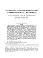
FIG. 1. Secondary Loan Market Volume.
Source: Reuters LPC Traders Survey.
Banks and other financial institutions have sold loans among themselves for over
100 years. Even though this market has existed for many years, it grew slowly until the
early 1980s when it entered a period of spectacular growth, largely due to expansion
in highly leveraged transaction (HLT) loans to finance leveraged buyouts (LBOs)
and mergers and acquisitions (M&As). With the decline in LBOs and M&As in the
late 1980s after the stock market crash of 1987, the volume of loan sales fell to
approximately $10 billion in 1990. However, since then the volume of loan sales
has expanded rapidly, especially as M&A activity picked up again.
3
Figure 1 shows
the rate of growth in the secondary market for loans from 1991 to 2007. Note that
secondary market loan transactions have exceeded $100 billion a year since 2000.
The secondary loan sales market is sometimes segmented based on the type of
investors involved on the “buy side,” for example, institutional loan market versus
retail loan market. An alternative way of stratifying loan trades in the secondary
market is to distinguish between the “par” loans (loans selling at 90% or more of face
value) and “distressed” loans (loans selling at below 90% of face value). Figure 1

also shows an increasing proportion of distressed loan sales, reaching approximately
42% of the total loan sales in 2002. However, the proportion of distressed loan sales
has come down to more moderate levels post-2002.
3. Specifically M&A activity increased from $190 billion in 1990 to $500 billion in 1995, and to over
$1,800 billion in 2000 (Thomson Financial Securities Data Corporation).
EDWARD I. ALTMAN, AMAR GANDE, AND ANTHONY SAUNDERS : 759
2. DATA AND SAMPLE SELECTION
The sample period for our empirical analysis is from November 1, 1999 to October
31, 2007. Our choice of sample period is driven by data considerations. That is, our
empirical analysis requires secondary market daily prices of loans, which were not
available prior to November 1, 1999. In addition, since the required data were not
available from a single source, we use multiple sources of data to construct a data set
for our empirical analysis. Furthermore, since these multiple data sources do not have
a unique identifier, we manually match using the company name and other identifying
variables, such as date. We next describe the construction of our data set from these
multiple sources of data.
We start with the database of daily secondary market loan prices. This is a new
database from the Loan Syndications and Trading Association (LSTA) and Loan Pric-
ing Corporation (LPC), supplied to over 100 institutions managing over $200 billion
in bank loan assets under the name “Secondary Market Pricing Service” (SMPS).
This database contains daily bid and ask price quotes aggregated across dealers. Each
loan has a minimum of at least two dealer quotes and a maximum of over 30 dealers,
including all top loan broker-dealers.
4
These price quotes are obtained on a daily basis
by LSTA in the late afternoon from the dealers. The items in this database include
a unique loan identification number (LIN); name of the issuer (Company); type of
loan, for example, term loan (Facility); date of pricing (Pricing Date); average of bid
quotes (Avg Bid); number of bid quotes (Bid Quotes); average of second and third
highest bid quote (High Bid Avg); average of ask quotes (Avg Ask); number of ask

quotes (Ask Quotes); and average of second and third lowest ask quotes (Low Ask
Avg).
For our empirical analysis, we also need daily secondary market bond prices.
However, we need the nine-character bond cusip assigned by Standard & Poor’s
to each bond to obtain daily secondary market bond prices from the data sources
mentioned below. We manually search the Fixed Income Securities Database (FISD)
using the name of the issuer in the SMPS database to match with the name of the
issuer in FISD to extract the relevant nine-character bond cusips.
We use two data sources for bond prices over two nonoverlapping subperiods that
together span our entire sample period. The main reason for doing this is an alternative
comprehensive database of bond prices, known as “Trade Reporting and Compliance
Engine” (TRACE) became available during the later part of the sample period as a
result of an improvement in bond market transparency.
5
The first data source for daily
bond prices is the Salomon (now Citigroup) Yield Book (YB). We extract daily bond
4. Since LSTA and LPC do not make a market in bank loans and are not directly or indirectly involved
in the buying or selling of bank loans, the LSTA/LPC mark-to-market pricing service is believed to be
independent and objective.
5. The National Association of Securities Dealers (NASD) phased-in the dissemination of bond trans-
action information through its TRACE initiative—in particular, prices—starting with an initial set of
investment grade bonds (about 500) in July 2002. The coverage was expanded to the full universe of bonds
(including high yield bonds) in October 2004.
760 : MONEY, CREDIT AND BANKING
prices from the YB database from November 1, 1999 to June 30, 2002 for all the
companies in the SMPS database using their nine-character bond cusips from FISD.
The second data source for daily bond prices is the TRACE database. We extract end
of day bond prices from TRACE from July 1, 2002 to October 31, 2007 for all the
companies in the SMPS database using their nine-character bond cusips from FISD.
We use the same data source in computing daily bond returns. For example, bond

returns calculated from TRACE start on July 2, 2002 since the first available bond
price in TRACE is on July 1, 2002.
Our loan defaults data come from Portfolio Management Data (PMD), a business
unit of Standard & Poor’s that has been tracking loan defaults in the institutional loan
market since 1995. We have confirmed with the data provider that these loan defaults
correspond to a missed interest or a principal payment rather than a technical violation
of a covenant. We manually match the company names from the loan defaults database
with the company names from the SMPS database for our empirical analysis.
Finally, we obtain information on security-specific characteristics (for the purpose
of reporting some descriptive statistics of our sample), such as size, maturity,seniority,
collateral, and covenants from the Dealscan database of the LPC for loans and from
the FISD for bonds. As before, due to the absence of a unique identifier that ties the
databases together, we merge these databases with the others by manually matching
based on the company name from the SMPS database.
3. TESTABLE HYPOTHESIS
Above, we have argued that banks as “insiders” have continued skills and incentives
to monitor their loans to a borrower even in the presence of an active secondary market
for bank loans. The resulting monitoring advantage of bank loans relative to public
bonds implies that secondary market loan prices will reflect any additional information
from such continued bank loan monitoring. In contrast, secondary market bond prices
do not reflect such “inside” information simply because bond investors do not have
similar inside informational access to a borrowing firm.
It could be argued that bond investors may be able to access secondary market loan
prices and thus piggyback on the incremental benefits of bank monitoring. Never-
theless, even if that were to be the case, a bond investor would still effectively lag a
loan investor in terms of new information. Consequently, the monitoring advantage
of bank loans relative to public bonds leads to the following testable hypothesis:
Secondary market loans are informationally more efficient than secondary market
bonds prior to a loan default date.
We empirically examine the above hypothesis in Section 4.1 through Granger-

causality tests based on vector autoregression (VAR) models of the daily returns in
the secondary market for loans and bonds. Specifically, we analyze whether loan
returns Granger cause bond returns and whether bond returns do not Granger cause
loan returns prior to a loan default date.
EDWARD I. ALTMAN, AMAR GANDE, AND ANTHONY SAUNDERS : 761
TABLE 1
D
ESCRIPTIVE STATISTICS
Loans Bonds Difference
Variable Mean t-stat Mean t-stat Mean t-stat
MATURITY (months) 60.98 30.63
∗∗∗
67.56 18.65
∗∗∗
−6.58 1.59
AMOUNT ($ million) 501.29 14.79
∗∗∗
408.88 21.57
∗∗∗
92.41 2.38
∗∗
SENIOR (fraction) 1.00 nm 0.95 56.98
∗∗∗
−0.05 −3.07
∗∗∗
SECURED (fraction) 0.70 20.43
∗∗∗
0.03 2.49
∗∗
0.67 18.06

∗∗∗
COVENANT SCCORE (0–4) 1.62 14.11
∗∗∗
2.99 46.63
∗∗∗
−1.37 −10.46
∗∗∗
NOTE: This table presents descriptive statistics of the 176 matched loan-bond pairs (based on the name of the borrower), making it a total of
352 observations. MATURITY stands for the remaining maturity (in months) of the loan or the bond, as on the loan default date of the same
company. AMOUNT stands for the amount of the loan or bond issue (in $ millions). SENIOR and SECURED each take a value of one if a loan
or a bond is classified likewise and zero otherwise. COVENANT SCORE is the sum of four dummy variables that represent four loan/bond
covenants as described in Smith and Warner (1979) and Bagnani et al. (1994), namely, INVCOV = 1 for restrictions on investments,
DIVCOV = 1 for restrictions on dividends, FINCOV = 1 for restrictions of financing, and PAYCOV = 1 for covenants modifying payoff to
investors. ** and *** stand for statistical significance at the 5% and 1% levels, respectively, using a two-tailed test, and nm refers to “not
meaningful.”
4. EMPIRICAL RESULTS
Table 1 presents descriptive statistics of matched loan-bond pair data (based on
the name of the borrower). Loans typically have a shorter maturity and are larger (in
terms of issue size) than bonds. Moreover, as is well known, loans are more senior
and are more secured than bonds.
6
We compute a daily loan return based on the midprice quote of a loan, namely, the
average of the bid and ask price of a loan in the loan price data set.
7
That is, a one-day
loan return is computed as today’s midprice divided by yesterday’s midprice of a loan
minus one. The daily bond returns are computed based on the prices of a bond in
the bond price data set in an analogous manner. During the July 2002–October 2007
sample period, where we use the TRACE bond transaction data, we compute daily
returns based on the last recorded price on any particular day.

4.1 Informational Efficiency of Loans versus Bonds
We investigate the informational efficiency of loans versus bonds using Granger
causality tests (see Granger 1969 and Sims 1972 for details). Empirically, we follow
the Hotchkiss and Ronen (2002) methodology, by conducting Granger causality tests
based on VAR models for the daily returns in the secondary market for loans and
bonds. Specifically, we equally weight secondary market loan returns and secondary
market bond returns of matched loan-bond pairs (based on the name of the borrower),
6. The relevance of collateral in debt financing is well established in the literature. For example,
Berger and Udell (1990, 1995) document that collateral plays an important role in more than two-thirds of
commercial and industrial loans in the United States. John, Lynch, and Puri (2003) study how collateral
affects bond yields. Also, see Dahiya, Saunders, and Srinivasan (2003) for more evidence on the value of
monitoring to a borrower.
7. We calculate returns based on the midprice to control for any bid–ask “bounce.” See, for example,
Stoll (2000) and Hasbrouck (1988) for more details.
762 : MONEY, CREDIT AND BANKING
and examine whether secondary market loan returns Granger cause secondary market
bond returns or whether secondary market bond returns Granger cause secondary
market loan returns during the preloan default period, that is, the time period leading
up to a loan default, such as [−244, −11], where day 0 refers to a loan default
date. For robustness, we consider several alternative preloan default periods, such
as [−244, −6], [−244, −1], [−122, −11], [−61, −11], and find that our results
(discussed later in this section) are invariant to the exact definition of the preloan
default period.
To test the null, that secondary market loan returns do not Granger cause secondary
market bond returns, following Hotchkiss and Ronen (2002), we rely on a bivariate
VAR model (equation (1)), and estimate by ordinary least squares (OLS):
RB
t
= c
1

+
j

i=1
a
1,i
RB
t−i
+
j

i=1
b
1,i
RL
t−i
+ ν
1,t
. (1)
Similarly, to test the null that secondary market bond returns do not Granger
cause secondary market loan returns, we rely on a similar bivariate VAR model
(equation (2)):
RL
t
= c
2
+
j

i=1

a
2,i
RL
t−i
+
j

i=1
b
2,i
RB
t−i
+ ν
2,t
, (2)
where RB
t
are the equally weighted secondary market bond returns, RL
t
are the
equally weighted secondary market loan returns, as and bs are OLS coefficient es-
timates, cs are the regression constants, ν
t
s are the disturbance terms, and j is the
lag length. We then conduct F-tests of the null hypothesis that secondary market
loan returns do not Granger cause secondary market bond returns using equation (3),
and of the null hypothesis that secondary market bond returns do not Granger cause
secondary market loan returns using equation (4):
H
0

: b
1,i
= 0, ∀i, (3)
H
0
: b
2,i
= 0, ∀i. (4)
Following Hamilton (1994) we test equations (3) and (4) using lag lengths from
1 to 10 days.
8
We do not make any assumption as to which of these lag lengths is
optimal, and draw inferences based on the overall evidence, rather than based on a
specific lag length.
Table 2 summarizes the results of the Granger causality tests prior to a loan default.
We find strong evidence that secondary market loan returns Granger cause secondary
8. For a similar approach, see Kwan (1996) who uses a lag length of 1 in analyzing the informational
efficiency of stocks versus bonds. Our approach uses a range of lags from 1 to 10, and is focused on the
informational efficiency of loans versus bonds.
EDWARD I. ALTMAN, AMAR GANDE, AND ANTHONY SAUNDERS : 763
TABLE 2
G
RANGER CAUSALITY TESTS USING A BIVARIATE VA R
Panel A. Expanded versions of the preloan default period
Preloan default period [−244, −11] Preloan default period [−244, −6] Preloan default period [−244, −1]
Loan returns Bond returns Loan returns Bond returns Loan returns Bond returns
do not do not do not do not do not do not
Null Granger cause Granger cause Granger cause Granger cause Granger cause Granger cause
hyp. bond returns loan returns bond returns loan returns bond returns loan returns
Lags F-statistic F-statistic F-statistic F-statistic F-statistic F-statistic

1 5.17
∗∗
0.28 4.57
∗∗
0.28 6.46
∗∗
0.56
2 4.97
∗∗∗
0.13 3.81
∗∗
0.18 3.96
∗∗
0.27
3 4.47
∗∗∗
0.13 3.02
∗∗
0.17 3.07
∗∗
0.23
4 3.46
∗∗∗
0.32 2.33
∗
0.37 2.33
∗
0.29
5 3.15
∗∗∗

0.26 2.04
∗
0.30 1.99
∗
0.23
6 2.69
∗∗
0.47 1.82
∗
0.46 1.69 0.46
7 2.58
∗∗
0.50 1.93
∗
0.45 1.78
∗
0.47
8 2.39
∗∗
0.80 1.75
∗
0.86 1.60 0.84
9 2.12
∗∗
0.85 1.55 0.92 1.41 0.93
10 1.95
∗∗
0.81 1.38 0.85 1.42 0.85
Panel B. Reduced versions of the preloan default period
Preloan default period [−244, −11] Preloan default period [−121, −11] Preloan default period [−61, −11]

Loan returns Bond returns Loan returns Bond returns Loan returns Bond returns
do not do not do not do not do not do not
Null Granger cause Granger cause Granger cause Granger cause Granger cause Granger cause
hyp. bond returns loan returns bond returns loan returns bond returns loan returns
Lags F-statistic F-statistic F-statistic F-statistic F-statistic F-statistic
1 5.17
∗∗
0.28 8.10
∗∗∗
6.16
∗∗
4.93
∗∗
3.23
∗
2 4.97
∗∗∗
0.13 4.52
∗∗
3.30
∗∗
3.69
∗∗
1.98
3 4.47
∗∗∗
0.13 3.68
∗∗
2.03 2.93
∗

1.52
4 3.46
∗∗∗
0.32 4.31
∗∗∗
1.66 3.51
∗∗
1.30
5 3.15
∗∗∗
0.26 3.76
∗∗∗
1.17 2.56
∗∗
0.99
6 2.69
∗∗
0.47 3.11
∗∗∗
1.16 2.04
∗
1.35
7 2.58
∗∗
0.50 2.65
∗∗
1.20 1.72 1.17
8 2.39
∗∗
0.80 2.52

∗∗
1.27 1.91
∗
0.96
9 2.12
∗∗
0.85 2.36
∗∗
1.25 1.84
∗
0.93
10 1.95
∗∗
0.81 2.45
∗∗
1.63 2.70
∗∗
1.61
NOTE: This table summarizes the results of Granger causality tests. Following Hotchkiss and Ronen (2002), we use equally weighted
loan returns and bond returns of 176 matched loan-bond pairs (based on the name of the borrower) prior to a loan default date of the
same company. Specifically, we conduct an F-test of the null hypothesis that the loan returns do not Granger cause the bond returns as
shown in equation (3). Similarly, we also conduct an F-test of the null hypothesis that the bond returns do not Granger cause the loan
returns as shown in equation (4). In Panel A, we present results separately for expanded versions of the preloan default period, namely,
[−244, −11], [−244, −6] and [−244, −1], and in Panel B, we present results separately for the reduced versions of the preloan default
period, namely, [−244, −11], [−121, −11] and [−61, −11], where day 0 refers to the loan default date.
∗
,
∗∗
, and
∗∗∗

stand for statisti-
cal significance of the reported F-statistic (in rejecting the null hypothesis of no Granger causality) at the 10%, 5%, and 1% levels, respectively.
market bond returns, independent of the number of lags. For example, the F-statistic
for the null hypothesis that daily secondary market loan returns have no explana-
tory power for the daily secondary market bond returns during the [−244, −11]
preloan default period (see equation (3)) in Panel A of Table 2 is 4.97 at a lag
length of 2 and 3.15 at a lag length of 5; both imply that the null hypothesis in
equation (3) is rejected at the 1% level. This evidence suggests that the secondary
764 : MONEY, CREDIT AND BANKING
market loan returns Granger cause secondary market bond returns prior to a loan
default date.
In contrast, we find no evidence that secondary market bond returns Granger cause
secondary market loan returns. For example, the F-statistic for the null hypothesis that
daily bond returns have no explanatory power for loan returns during the [−244, −11]
preloan default period (see equation (4)) in Panel A of Table 2 is 0.13 at a lag length
of 2 and 0.26 at a lag length of 5; both imply that the null hypothesis in equation (4)
cannot be rejected at any reasonable level of significance. This evidence suggests that
secondary market bond returns do not Granger cause secondary market loan returns
prior to a loan default date.
In summary, we find strong evidence supporting the informational efficiency hy-
pothesis specified in Section 3. That is, consistent with a monitoring advantage of loans
over bonds, we find evidence that secondary market loan returns Granger cause sec-
ondary market bond returns, whereas secondary market bond returns do not Granger
cause secondary market loan returns prior to a loan default. We next examine the
robustness of this finding to different definitions of the preloan default period, and
in the extent to which this finding is influenced by sample companies with multiple
loans or bonds.
Preloan default period. Our result that prior to a loan default, secondary market loan
returns Granger cause secondary market bond returns whereas secondary market bond
returns do not Granger cause secondary market loan returns, is based on a preloan

default period defined as [−244, −11], where day 0 refers to a loan default date. We
now examine whether this result changes if we change the definition of the preloan
default period.
First, we examine whether we obtain the same result if we expand the length of the
preloan default period from [−244, −11] to [−244, −6] and [−244, −1]. Panel A
of Table 2 presents, in addition to the results corresponding to [−244, −11], the
results for the expanded versions of the preloan default period (i.e., [−244, −6] and
[−244, −1])). The results for the [−244, −6] and [−244, −1] periods are qualitatively
similar to that of the [−244, −11] period.
Second, we examine whether we obtain the same result if we reduce the length of the
preloan default period from [−244, −11] to [−121, −11] and [−61, −11]. Panel B
of Table 2 presents the results for the reduced versions of the preloan default period
(i.e., [−121, −11] and [−61, −11]) for comparison with that of [−244, −11]. Once
again, the results are qualitatively unchanged. In particular, while loan returns Granger
cause bond returns at almost all lag lengths, bond returns do not Granger cause
loan returns, with the exception of the first two lags. Hence, for the remainder of
the analysis, we focus only on the expanded versions of the preloan default period,
namely, [−244, −11], [−244, −6], and [−244, −1].
Multiple loans or bonds for the same company. Given that some companies in our
sample have multiple loans or bonds, equally weighting returns in our Granger causal-
ity tests implicitly results in a proportionately larger weight for such companies.
To that extent, one could argue that our major result, that prior to a loan default,
EDWARD I. ALTMAN, AMAR GANDE, AND ANTHONY SAUNDERS : 765
TABLE 3
G
RANGER CAUSALITY TESTS USING A BIVARIATE VA R ( A CCOUNTS FOR MULTIPLE LOANS OR BONDS OF THE SAME
BORROWER)
Preloan default period [−244, −11] Preloan default period [−244, −6] Preloan default period [−244, −1]
Loan returns Bond returns Loan returns Bond returns Loan returns Bond returns
do not do not do not do not do not do not

Null Granger cause Granger cause Granger cause Granger cause Granger cause Granger cause
hyp. bond returns loan returns bond returns loan returns bond returns loan returns
Lags F-statistic F-statistic F-statistic F-statistic F-statistic F-statistic
1 0.27 0.26 0.16 0.04 1.37 0.12
2 0.23 2.79
∗
0.37 2.92
∗
1.97 1.61
3 1.42 1.96 0.52 2.08 2.03 1.16
4 1.71 1.46 1.81 1.54 3.61
∗∗∗
0.85
5 2.86
∗∗
1.74 2.58
∗∗
1.78 3.78
∗∗∗
1.93
∗
6 2.34
∗∗
1.52 2.27
∗∗
1.56 3.12
∗∗∗
2.01
∗
7 2.07

∗∗
1.31 1.97
∗
1.34 2.72
∗∗∗
1.78
∗
8 1.80
∗
1.22 1.75
∗
1.27 2.44
∗∗
1.68
9 1.78
∗
1.23 1.74
∗
1.24 2.28
∗∗
1.59
10 2.40
∗∗
1.16 2.21
∗∗
1.19 2.67
∗∗∗
1.52
NOTE: This table summarizes the results of Granger causality tests. Following Hotchkiss and Ronen (2002), we use equally weighted loan
returns and bond returns of 176 matched loan-bond pairs (based on the name of the borrower) prior to a loan default date of the same

company. If a company has multiple loan-bond pairs, we choose the loan-bond pair that has the maximum number of observations among
all the loan-bond pairs for the same company in the equal weighting across companies, thus ensuring that every company receives the same
weight in constructing the portfolio returns. Specifically, we conduct an F-test of the null hypothesis that the loan returns do not Granger
cause the bond returns as shown in equation (3). Similarly, we also conduct an F-test of the null hypothesis that the bond returns do not
Granger cause the loan returns as shown in equation (4). We present results separately for the expanded versions of the preloan default
period, namely [−244, −11], [−244, −6], and [−244, −1], where day 0 refers to the loan default date.
∗
,
∗∗
, and
∗∗∗
stand for statisti-
cal significance of the reported F-statistic (in rejecting the null hypothesis of no Granger causality) at the 10%, 5%, and 1% levels, respectively.
secondary market loan returns Granger cause secondary market bond returns, whereas
secondary market bond returns do not Granger cause secondary market loan returns,
may be disproportionately driven by companies with multiple loans or bonds.
To address whether our result is susceptible to the above-mentioned bias, we modify
our Granger causality analysis by selecting a single loan-bond pair for each company
before we equally weight the returns. Specifically, for companies with multiple loan-
bond pairs, we select the loan-bond pair that has the most number of total (i.e., bond
plus loan) return observations during the preloan default period. We then equally
weight the returns as before. Thus, our modified analysis ensures that each company
gets an equal weight in the Granger causality analysis, independent of whether or not
it has multiple loans or bonds that are traded.
We modify our analysis as described above and rerun the regression analysis for the
expanded versions of the preloan default period, namely, [−244, −11], [−244, −6],
and [−244, −1] of Table 2. The results of the modified analysis are presented in
Table 3. The results are once again qualitatively similar to those in Table 2. That
is, prior to a loan default, there is a substantial amount of evidence of loan returns
Granger causing bond returns, whereas there is very little evidence of bond returns

Granger causing loan returns.
Based on the above evidence, we conclude that the secondary loan market is infor-
mationally more efficient than the secondary bond market prior to a loan default date
766 : MONEY, CREDIT AND BANKING
and that this conclusion is independent of the specificdefinition of the preloan default
period and is not entirely driven by sample companies that have multiple loans or
bonds.
5. CONCLUSIONS
Using a new data set of secondary market prices of corporate loans, we find the
secondary loan market to be informationally more efficient than the secondary bond
market prior to a loan default. Specifically, we find that secondary market loan returns
Granger cause secondary market bond returns prior to a loan default. In contrast,
secondary market bond returns do not Granger cause secondary market loan returns
prior to a loan default.
Overall, our results have important implications regarding the continuing special-
ness of banks as monitors and the benefits of loan monitoring for other financial
markets, such as the bond market.
LITERATURE CITED
Angbazo, Lazarus A., Jianping Mei, and Anthony Saunders. (1998) “Credit Spreads in the
Market for Highly Leveraged Transaction Loans.” Journal of Banking and Finance, 22,
1249–82.
Bagnani, Elizabeth S., Nikolaos T. Milonas, Anthony Saunders, and Nickolaos G. Travlos.
(1994) “Managers, Owners, and the Pricing of Risky Debt: An Empirical Analysis.” Journal
of Finance, 49, 453–77.
Berger, Allen N., and Gregory F. Udell. (1990) “Collateral, Loan Quality, and Bank Risk.”
Journal of Monetary Economics, 25, 21–42.
Berger, Allen N., and Gregory F. Udell. (1995) “Relationship Lending and Lines of Credit in
Small Firm Finance.” Journal of Business, 68, 351–81.
Dahiya, Sandeep, Anthony Saunders, and Anand Srinivasan. (2003) “Financial Distress and
Bank Lending Relationships.” Journal of Finance, 58, 375–99.

Diamond, Douglas W. (1984) “Financial Intermediation and Delegated Monitoring.” Review
of Economic Studies, 51, 393–414.
Drucker, Steven, and Manju Puri. (2009) “On Loan Sales, Loan Contracting, and Lending
Relationships.” Review of Financial Studies, 22, 2835–72.
Fama, Eugene F. (1985) “What’s Different about Banks?” Journal of Monetary Economics,
15, 29–39.
Gorton, Gary, and George G. Pennacchi. (1995) “Banks and Loan Sales: Marketing Non-
marketable Assets.” Journal of Monetary Economics, 35, 389–411.
Granger, Clive W. J. (1969) “Investigating Causal Relations by Econometric Models and Cross-
Spectral Methods.” Econometrica, 37, 424–38.
Hamilton, James D. (1994) Time Series Analysis. Princeton, NJ: Princeton University Press.
EDWARD I. ALTMAN, AMAR GANDE, AND ANTHONY SAUNDERS : 767
Hasbrouck, Joel. (1988) “Trades, Quotes, Inventories, and Information.” Journal of Financial
Economics, 22, 229–52.
Hotchkiss, Edith S., and Tavy Ronen. (2002) “The Informational Efficiency of the Corporate
Bond Market: An Intraday Analysis.” Review of Financial Studies, 15, 1325–54.
John, Kose, Anthony W. Lynch, and Manju Puri. (2003) “Credit Ratings, Collateral, and Loan
Characteristics: Implications for Yield.” Journal of Business, 76, 371–409.
Kroszner, Randall S., and Philip E. Strahan. (2001) “Throwing Good Money after Bad? Board
Connections and Conflicts in Bank Lending.” NBER Working Paper No. 8694.
Kwan, Simon H. (1996) “Firm-specific Information and Correlation between Individual Stocks
and Bonds.” Journal of Financial Economics, 40, 63–80.
Ramakrishnan, Ram T. S., and Anjan V. Thakor. (1984) “Information Reliability and a Theory
of Financial Intermediation.” Review of Economic Studies, 51, 415–32.
Saunders, Anthony, and Marcia M. Cornett. (2008) Financial Institutions Management: A Risk
Management Approach, 6th ed. New York, NY: McGraw-Hill Publishers.
Sims, Christopher A. (1972) “Money, Income and Causality.” American Economic Review, 62,
540–52.
Smith, Clifford W., and Jerold B. Warner. (1979) “On Financial Contracting: An Analysis of
Bond Covenants.” Journal of Financial Economics, 7, 117–61.

Stoll, Hans R. (2000) “Friction.” Journal of Finance, 55, 1479–514.