Measurement, Monitoring, and Forecasting of Consumer Credit Default Risk – An Indicator Approach Based on Individual Payment Histories doc
Bạn đang xem bản rút gọn của tài liệu. Xem và tải ngay bản đầy đủ của tài liệu tại đây (850.49 KB, 29 trang )
SCHUMPETER DISCUSSION PAPERS
Measurement, Monitoring, and Forecasting of
Consumer Credit Default Risk –
An Indicator Approach Based on Individual Payment Histories
Alexandra Schwarz
SDP 2011-004
ISSN 1867-5352
© by the author
Measurement, Monitoring and Forecasting of
Consumer Credit Default Risk
∗
An Indicator Approach
Based on Individual Payment Histories
Alexandra Schwarz
German Institute for International Educational Research
Frankfurt am Main, Germany
Abstract
The statistical techniques which cover the process of modeling and evaluating
consumer credit risk have become widely accepted instruments in risk management.
In contrast, we find only few and vague statements on how to define the default
event, i. e. on the concrete circumstances that lead to the decision of identifying a
certain credit as defaulted. Based on a large data set of individual payment histories
this paper investigates a possible solution to this problem in the area of installment
purchase. The proposed definition of default is based on the time due amounts are
outstanding and the resulting profitability of the receivables portfolio. Furthermore,
to assess the individual payment performance during the credit period, indicators for
monitoring and forecasting default events are derived. The empirical results show
that these indicators generate valuable information which can be used by the creditor
to improve his credit and collection policy and hence, to improve cash flows and
reduce bad debt loss.
Keywords: Credit Risk Analysis · Credit Default · Risk Management · Accounts Receiv-
able Management · Performance Measurement
JEL Classification: C44 · G32 · M21
∗
The author gratefully acknowledges the support of Gerhard Arminger (University of Wuppertal) and
helpful comments of Annette K
¨
ohler (University of Duisburg-Essen) and participants at the 4th European
Risk Conference in Nottingham, September 2010.
1
SCHUMPETER DISCUSSION PAPERS 2011-004
1 Introduction
In theory, a Good account is one that you are glad you took
and a Bad account is one that you are sorry you took.
That may be true but isn’t very helpful.
(Edward M. Lewis, 1992)
Offering customers installment purchase is a widely-used instrument to increase sales.
For the firm implementing this instrument, payment by installments is a sale on credit
with special conditions, especially including an extended credit period and an installment
plan fixing the due dates for payments to be made by the customer. Sales on credit as
one part of a selling concept, directly incorporate a conflict between marketing and finan-
cial objectives – between gaining customers and controlling the credit risk involved by
extended, more customer-oriented payment conditions.
The operative control of these credits is assigned to accounts receivable management
whose key tasks are to record and manage payments, to configure terms of payment and
trading conditions, to induce collection procedures and to control loan securities, if avail-
able.
1
As every such credit involves a default risk, an effective receivables management
aims for preventing bad debt loss and should therefore check the customers’ creditwor-
thiness (Hoss 2006, 35; Johnson/Kallberg 1986, 9 ff.). The analysis and prediction of
this default risk is usually supported by a standardized process, often referred to as credit
scoring. This process is based on statistical methods for estimating the individual prob-
abilities of customers to default on credit which are one of the essential inputs for the
financial evaluation of credit sales and of the impact these sales have on a firm’s working
capital and liquidity.
The techniques that cover the process of modeling individual credit risks are widely dis-
cussed topics in financial and statistical literature.
2
In contrast, we find only few state-
ments on how the dependent variable default yes/no in a scoring model is defined. Even
in statistical publications this definition is always said to be given, but not described.
Nonetheless, defining credit default events is a critical task within the process of model-
ing credit risk as any such definition is needed to operationalize the key dependent variable
(e. g. creditworthiness), to calculate default probabilities and to monitor them over time.
1
See Brigham (1992), Johnson/Kallberg (1986) and Mueller-Wiedenhorn (2006) for an introduction to
accounts receivable management.
2
For an introduction to these techniques see for example Caouette et al. (2008, 201 ff.), Hand/Henley
(1997) and Thomas et al. (2002).
2
SCHUMPETER DISCUSSION PAPERS 2011-004
It can be assumed that this lack of information is due to confidentiality reasons because
the definition of credit default gives direct insight into a bank’s or a company’s internal
calculations, its marketing strategy and credit policy.
The present paper addresses this question as it deals with the definition, monitoring and
forecasting of default events in the area of installment credits. The focus is on two ques-
tions:
(1) How can a credit default event be defined? That is, what are the concrete circum-
stances, e. g. in terms of payment behavior, that lead to the decision of classifying a
certain account as defaulted?
(2) What are useful indicators for monitoring individual payment behavior and detecting
default events during the payment process?
Hence, the paper is organized as follows: First, the credit scoring process is set in the
context of risk analysis in section 2 where the information generated by a credit scoring
system and its implications for accounts receivable and credit risk management are de-
scribed. Section 3 deals with the need for defining credit default. We review and discuss
existing definitions of default events and describe general characteristics any definition of
credit default should fulfill. To arrive at a possible definition of credit default, the patterns
of payment – a common measure for the control of accounts receivable – are adopted to
the case of installment purchase (section 4). Events of default and non-default are classi-
fied based on a measure of profitability that can be derived from these payment patterns.
In the empirical study, this approach is applied to a large, unique data set of payment
histories originating from a company trading consumer goods. Section 5 deals with indi-
cators of individual payment performance and the monitoring of payment behavior. The
empirical study continues by evaluating the proposed indicators with respect to their po-
tential to detect defaults on-line, i. e. during the payment process. The paper closes with
a discussion in section 6.
3
SCHUMPETER DISCUSSION PAPERS 2011-004
2 Credit scoring systems for evaluating sales on credit
In the ideal case, a credit scoring system for identifying, analyzing and monitoring cus-
tomer credit risk is an integrative part of a company’s risk management: on the one hand
such a system depends on historical accounting data, on the other hand it generates useful
information for controlling and managing credit risk. Consequently, evaluating sales on
credit by means of a scoring system is a concurrent process as illustrated in figure 1.
To measure the default risk involved by sales on credit, customers are assigned to certain
risk classes based on their individual propensities to default on payment. The required
default probability can either be obtained externally or on basis of an internal scoring
model. The main internal source of information on creditworthiness is a company’s own
accounting department which can provide data on a customer’s previous payment behav-
ior and individual characteristics like age, education, profession, residence etc. By means
of statistical methods, this data can be used to construct and estimate a credit scoring
model for the prediction of the default probability of new credits. Firms can also turn
to commercial credit agencies which collect data on contractual and non-contractual pro-
cessing of business connections. Companies which provide goods and services on credit
can purchase information on criteria like outstanding accounts, requests to pay issued by
court order, enforcement procedures and uncovered checks. These criteria normally serve
as knock-out criteria as they deliver outright facts on a consumer’s propensity to default
on payment (Reichling et al. 2007, 56). Following the design of corporate ratings, some
credit agencies provide consumer ratings. These are individual score point values which
are assigned a certain default probability. Such an external credit score can also be used
as an additional input feature in an internally developed credit scoring model.
Independent of the source of credit quality information, the next step consists in defining
risk classes and in establishing decisions with respect to credit applications. In this re-
gard, cut-off values have to be defined on the ordinal or metric default probability scale.
Besides the number of risk classes this requires the systematic formulation of activities
to be taken on customers who are assigned to a certain risk class. A simple example
would be to establish two risk classes representing sufficient and insufficient payment,
or creditworthy and not creditworthy customers, respectively. To avoid the involved
risk, a firm’s risk management may decide to refuse applications of customers who are
not creditworthy. As firms always bear the risk involved by accepted sales on credit,
more diversified risk strategies lead to a range of classes and interventions, accompa-
nied by risk-based pricing, adjustment of payment terms and risk-adjusted interest rates.
4
SCHUMPETER DISCUSSION PAPERS 2011-004
Figure 1: Process of implementing a credit scoring system
- Preliminary processes
- Definition of default/non-default
- Consolidation of internal data
and external information
- Construction and estimation
of a statistical credit scoring model
- Determination of cut-off value(s) on the default probability
scale
- Assignment of applicants to risk classes
- Class-dependent decision rules
- Refusal/conclusion of contract
- Risk-based adjustment of payment terms
-
Evaluation and calibration
Back-testing of obtained credit scoring system
(credit score, classification, and managerial advice)
Practical implementation
of credit scoring in risk management
Monitoring
of debtor/credit data and payment behavior
Externally
obtained
credit score
Development of an internal credit score
Estimated default probability
Definition of risk classes and related decisions
development feedback
processing feedback
Of course, the appropriate policy will be found by evaluating the profitability of alternative
systems, that is, by assessing the benefit of increased sales against the direct and indirect
costs of granting credit to customers with a varying likelihood to pay slowly or even end
up as a bad debt loss (Brigham 1992, 799).
Whether the obtained credit scoring really fulfills the desired targets is evaluated by back-
testing the whole system (scores, classifications and interventions) on the basis of a hold-
5
SCHUMPETER DISCUSSION PAPERS 2011-004
out sample of historical customer data. This calibration of the credit scoring provides
useful hints for the improvement of the developed model and the resulting decisions (de-
velopment feedback). Once the credit scoring has been implemented as part of the risk
management it is necessary to document the debtor- and credit-related data as well as
the individual processes of payment. This monitoring enables the technical and statis-
tical maintenance of the scoring model and it allows for a concurrent evaluation of the
risk involved by receivables, especially with respect to financing costs which reduce the
firm’s rate of return and liquidity (processing feedback). If, for example, slow or deficient
payments exceed a certain level, this may force the firm to adjust its credit policy, e. g. it
may increase the required financial strength of acceptable customers, or it may introduce
a more insistent collection policy.
3 On the definition of credit default events
This section deals with the general concept of credit default and the definition of credit
default events. It is discussed why it is inevitable to define the default event in a concrete
context, e. g. consumer credits offered by a bank or installment purchases offered by a
company, even if credit quality information is obtained externally. Afterwards, we review
existing definitions of default events and summarize their general characteristics.
3.1 The need for defining the credit default event
In contrast to default risk in general and the statistical techniques that cover the process
of modeling individual credit risks, the task of defining a credit as default or non-default
is only rarely discussed so far. Nonetheless, from a methodological point of view, there
are three main reasons why any such definition is strongly required in credit risk analysis.
First, if a firm
3
decides to establish its own internal credit scoring model, an operational-
ization of the latent dependent variable ‘creditworthiness’ is required. As creditors seek
for an estimation of default probability the dependent variable Z normally is binary coded,
i. e. Z ∈ (0, 1). Then z
i
= 1 represents a bad account and a not creditworthy customer,
and z
i
= 0 represents a good account and a creditworthy customer, respectively. Second,
even if a scoring system is based on an externally obtained credit score to predict indi-
vidual default risk, it is necessary to evaluate whether the obtained score really measures
what it is supposed to, i. e. if it really fits the individual credit risks of the customers at
3
As throughout the whole paper, the focus is on non-banks. Yet, the described concepts of credit default
and default events apply to banks as well, especially to the retail sector.
6
SCHUMPETER DISCUSSION PAPERS 2011-004
hand. The comparison of predicted and actual default risks requires an internal risk esti-
mator like default rates and therefore a definition of default and non-default. Finally, the
same reasoning applies to the validation of a scoring system once it has been implemented
for practical use. By monitoring the customers’ payment behavior and the appearance of
default events, firms are able to appraise whether the internal or external credit risk model
still fits the portfolio of customers at hand, and if the introduced business concept and
credit policy are still affordable.
3.2 A review of default event definitions
Most generally speaking, a bad account is a matter of deficient payment. A consistent
concept of the concrete circumstances which lead to the identification of a credit default
does not exist: “Even deciding on the definition of what should be regarded as a good
or bad risk may be far from straightforward.” (Hand 1998, 71) In addition, Hand points
out that the definition depends on the nature of the loan, i. e. the definitions of default
will be different for a credit card account and the repayment of a mortgage loan. “The
definition may be based on slow repayments (but is one month overdue to be regarded
as ‘bad’ or should it be two, or ?), a combination of account balance below some level
throughout the month and overdraft limit exceeded at some point, or some more sophisti-
cated combination.” (Hand 1998, 71) An indicator originating from the accounts receiv-
able management process may be the institution of legal proceedings against the debtor
(Fueser 2001, 45). Caouette et al. (2008, 208) suggest that the definition of a bad account
is usually based on three payment delinquencies whereas good accounts are those who
have not experienced these arrears. Lewis (1992) discusses the definition of credit default
with respect to revolving credit like credit card or bank giro accounts. He suggests that in
this context a good account “might be someone whose billing account shows:
(1) On the books for a minimum of 10 months.
(2) Activity in six of the most recent 10 months.
(3) Purchases of more than $50 in at least three of the past 24 months.
(4) Not more than once 30 days delinquent in the past 24 months.” (Lewis 1992, 36)
Here definitions (1) to (3) exclude those accounts from further investigations which be-
long to fairly new customers or to customers with low activity. Lewis (1992, 37) argues
that a bad account is more difficult to describe but may be identified adequately by one of
the following definitions:
7
SCHUMPETER DISCUSSION PAPERS 2011-004
– The debtor is delinquent for 90 days at any time with an outstanding undisputed bal-
ance of $50 or more.
– The debtor is delinquent three times for 60 days in the past 12 months with an out-
standing undisputed balance on each occasion of $50 or more.
– The debtor has gone bankrupt while the account was open.
According to Lewis, it is important to leave some accounts indeterminate, namely those
that do not fall in either group, because the lender may not be able to make a qualitative
decision on the performance of the loan, for example for newly acquired accounts or
accounts that are delinquent for 30 days.
An alternative approach to arrive at a definition of credit default may be to adopt the
definitions settled for banks by the Basel Committee on Banking Supervision (BCBS
2004, sect. 452). Within this framework two alternative definitions of default are given:
4
– Unlikeliness to pay: The bank considers that the obligor is unlikely to pay his/her credit
obligations to the banking group in full, without recourse by the bank to actions such
as realizing security (if held).
– 90 days past due: The obligor is past due more than 90 days on any essential credit
obligation.
Section 125 of the German Solvency Regulations (Deutsche Bundesbank 2008) con-
cretizes the unlikeliness-to-pay clause by a list of indicators which may suggest the def-
inition of default event, for example allowances for declined credit quality, sale of credit
obligations with a substantial economic loss, or the debtor has gone bankrupt. In this
regulation also the essential credit obligation mentioned in the 90-days-past-due clause
is specified more precisely. An overdraft of any obligation is said to be essential if it
amounts to more than 100 Euros and to more than 2.5% of the overall credit line. At
least the 90-days-past-due clause provides a precise definition of default events, but has
some fundamental drawbacks. These result from the fact that the Basel regulations, in-
cluding the definition of default events, were set to harmonize the measurement of capital
requirement. Hence great emphasis is placed on the evaluation of corporate credit, which
makes up the bulk of banks’ business. Therefore, the Basel 90-days-past-due clause need
not necessarily lead to an adequate decision on default events in terms of profitable or not
profitable accounts. Porath (2006), who discusses whether credit scoring models comply
4
These definitions are still valid in the ‘International framework for liquidity risk measurement, stan-
dards and monitoring’ (BCBS 2010).
8
SCHUMPETER DISCUSSION PAPERS 2011-004
with the Basel II requirements for risk quantification, argues that a scoring model’s pri-
mary aim is to support internal decisions and not to fulfill the supervisory requirements.
Consequently, “the default event sets as soon as the loan becomes no longer profitable for
the bank and this is usually not the case when the loan defaults according to the Basel
definition. It depends, instead, on the bank’s internal calculation.” (Porath 2006, 31) Ob-
viously, it can be assumed that the same applies to creditors in non-financial business and
it would be interesting to examine whether a company’s own definition of default events
goes in line with the Basel one.
The existing definitions of default events are either formulated in a very general manner,
or in case they are more precise they refer to a special type of loan like revolving credit.
From a managerial point of view this result is quite obvious: Every company has to arrive
at its own definition of default, depending on the nature of the loans and the company’s
internal calculation, its marketing strategy and credit policy. Consequently, the lack of
information on any concrete definition of default is due to confidentiality reasons and the
increased competition companies face in the industrial and commercial sector. This con-
clusion goes in line with Foster/Stine (2004) who build a predictive model for bankruptcy
and claim that their research, especially with respect to the identification of relevant pre-
dictors, suffers from issues of confidentiality in the credit industry and from the resulting
lack of exchange with credit analysts.
3.3 General characteristics of default event definitions
Based on the approaches reviewed above we can describe some general characteristics of
a default event definition. At first, there are basic requirements that should be considered
when developing a default definition.
– The definition of an account as good or bad is entirely based on the performance of
the account once accepted (Lewis 1992, 31). This means that the evaluation of per-
formance is only based on internal data concerning the individual payment process.
External information on credit quality or the application itself (e.g. age, profession etc.
of the credit applicant) is not included.
– The analysis of payment performance must lead to a definition that is consistent, pre-
cise and understandable, for the staff working with it as well as for internal and external
reviewers (Fueser 2001, 45; Lewis 1992, 36).
– The definition should offer the opportunity of a computer-aided, automated detection
of bad accounts (Lewis 1992, 37).
9
SCHUMPETER DISCUSSION PAPERS 2011-004
In addition, the more sophisticated methods of defining credit default, documented by the
BCBS (2004) and Lewis (1992), agree on two major components used for defining default
events.
(1) The temporal component: The customer is in arrears for a certain number of periods
(e. g. for 30 days). This means he failed to pay at a due date in the past.
(2) The monetary component: The customer is in arrears with a certain amount of money
(e. g. 100 Euros). This means he failed to pay at least one due amount in the past.
Independent of the type of loan, like revolving credit or installment purchase, these two
components of deficient payment induce different types of additional costs concerning an
accepted and open loan contract (Lauer 1998, 84 ff.; Salek 2005, 22):
– Every delayed payment induces additional costs in terms of interest charges for financ-
ing the capital fixed in outstanding accounts receivable.
– If outstanding amounts are not paid in the long run, this induces additional costs in
terms of bad debt loss.
– Both delayed payments and payments never made cause additional costs of managing
accounts receivable, not only overhead costs, but also costs of trying to collect accounts
receivable individually.
These general characteristics and components of default event definitions form the basis
of the approach to the classification of installment credits which is proposed in this paper.
4 A payment-pattern approach to the definition of credit
default events on aggregate level
A credit in the special form of an installment purchase usually involves an installment plan
which documents the due dates and due amounts of payment. These due and expected
payments can be compared to the actual payments of a debtor by means of the individual
account balances. The basic idea of the proposed classification is to balance expected and
actual payments of debtors on an aggregate level (e. g. on company level) at every point
in time at which payments are expected. By evaluating this pattern of payments and the
resulting profitability of the involved accounts we can determine the maximum period of
deficient payment which is acceptable for financial purposes.
10
SCHUMPETER DISCUSSION PAPERS 2011-004
4.1 Common approaches to the evaluation of accounts receivable
Most approaches to the control of accounts receivable follow a one-parameter technique:
A single indicator is used to describe the current status of the portfolio of accounts re-
ceivable and to forecast its development in the near future. Well-known examples are the
average days that sales are outstanding (DSO) and the reciprocal, i. e. the accounts receiv-
able turnover (ART), which gives the number of times that receivables will turn over in
one year (Johnson/Kallberg 1986, 28; Brigham 1992, 794 ff.; Lauer 1998, 57 ff.). Com-
puted on a monthly basis, increasing values of DSO and ART may suggest problems in
collecting receivables. To gain further insight into the composition of receivables one can
calculate an aging schedule which is the proportion of accounts receivable that are in dif-
ferent age classes (Stone 1976, 70). To control the development of accounts receivable,
any of these indicators is projected into the future, and to incorporate seasonal varying
sales on credit, the aging schedule of a certain month may be compared to the respective
aging schedule of the year before. More sophisticated methods, e. g. mover-stayer models
or Markov chain approaches, estimate the probabilities of accounts to change their state,
for example to make transitions among the state ‘paid’ and the state ‘overdue’. Frydman
et al. (1985) describe the application of both techniques to credit behavior. The result of
these procedures is an estimated transition matrix which gives these probabilities for the
total portfolio of analyzed accounts. The complexity of this procedure and the resulting
transition matrix increases rapidly with the number of states defined, especially if not only
states but also monetary components like outstanding amounts are considered.
5
The main drawback of these approaches with regard to defining default events is that all
of them give a more or less deep insight into the composition and the development of the
portfolio of accounts or customers, respectively. This is due to the fact that the emphasis
lays on once-only sales on credit which have to be paid until a certain payment deadline.
In addition, the analysis of accounts receivable aims for an appropriate estimation of
expected loss needed for a company’s annual balance. Consequently, neither the analysis
nor the control and forecasting of accounts receivable status refer to individual payment
behavior. Nonetheless, we make use of the patterns of payment – an alternative way to
measure the status and development of accounts receivable – to analyze payment behavior
and derive a profit-oriented definition of credit default events.
5
See for example the analysis described by Kallberg/Saunders (1983).
11
SCHUMPETER DISCUSSION PAPERS 2011-004
4.2 The patterns of payment
The patterns of payment are closely related to the aging schedule mentioned above. Their
main advantage over the previously described techniques is that they can be adopted ade-
quately to the case of installment credits. At the same time, they offer the opportunity to
assess the profitability of the accounts receivable portfolio.
In the context of sales on credit the receivable balance pattern “is the proportion of any
month’s sales that remains outstanding at the end of each subsequent month” (John-
son/Kallberg 1986, 25). This proportion is expected to decay over subsequent months.
Therefore, it is tracked by simply following the percentages over time. The collection
pattern is the mirror image of the receivable balance pattern, giving the cumulative col-
lections of the subsequent months in percent of credit sales. In the following, we define
suitable patterns of payment for the case of installment credits. A description of the orig-
inal procedures is given in Stone (1976).
Suppose we observe the complete payment history of n installment credits i = 1, . . . , n
with total financed amounts y
i
. We also suppose that these credits are paid off by an equal
number T of installments and that payments are due at regular intervals. Hence, payments
are observed at points in time t = 1, . . . , T, . . . , T + h, . . . , T + H with every t denoting
an observation point of due installments. Then T denotes the total number of installments
and at the same time the end of the agreed credit period, and H is the number of points
in time h = 1, . . . , H at which we observe payments after the end of the regular payment
term. Hence, T + H describes the end of our complete observation period.
Let y
i,t
denote the due amount of payment of credit i at time t, which is the installment to
be paid at time t, and let x
i,t
denote the respective amount actually paid at time t. Then
X
k
=
k
t=1
x
t
with x
t
=
n
i=1
x
i,t
(1)
are the cumulated payments actually made until k with k ∈ {1, . . . , T +H}. Equivalently,
the cumulated expected payments until k are denoted by
Y
k
=
k
t=1
y
t
with y
t
=
n
i=1
y
i,t
(2)
Consequently,
∆
k
=
k
t=1
δ
t
with δ
t
=
n
i=1
(y
i,t
− x
i,t
) (3)
12
SCHUMPETER DISCUSSION PAPERS 2011-004
are the cumulated outstanding payments at time k. Obviously, Y
k
= X
k
+ ∆
k
at each
k. In this retrospective analysis of payments the collection pattern over T + H points of
observation can be calculated as the respective cumulated payments in % of the overall
financed amount Y =
T
t=1
y
t
, i. e. X
k
/Y for all k. Respectively, the receivable balance
pattern is given by ∆
k
/Y , that are the respective cumulated outstanding amounts in % of
the total expected payment.
4.3 Measurement of profitability
The proposed definition of credit default events is based on the profitability of accounts
which can be measured using the patterns of payment described above. To illustrate this
approach we assume that an account is (still) profitable at time k if the additional costs
caused by deficient payment that occurred up to k are strictly smaller than the profit
generated by payments made up to k. For measuring the profitability P
k
of accounts at
time k, we introduce a weight a (in %) for the cumulated payments and a weight c (in
%) for the cumulated outstanding amounts ∆
k
. Then a · X
k
measures the profit made by
the payments received until time k, and c · ∆
k
denotes the additional costs caused by the
amounts not collected until time k. Then the profitability of the credit granting concept
can be measured by the indicator
P
k
= a · X
k
−
k
t=1
c · ∆
k
(4)
In addition, the weighted cumulated additional costs
k
t=1
c·∆
k
incorporate the so-called
revolving effect of credit which occurs if deficient payments are protracted over a certain
period. Let t
∗
denote the minimum k of all observation points for which P
k
≤ 0:
t
∗
= min
k=1, ,T +H
(k |P
k
≤ 0) (5)
This means, t
∗
is the point in time of the period of deficient payments at which the per-
formance of credits is no longer acceptable, whereas t
∗
− 1 denotes the last point in time
of the period of acceptable performance. This leads to the following classification rule
concerning the definition of the default event Z: Credit i is assigned to the class of bad
accounts if it contributes to the overall loss, that is, it shows an outstanding amount at t
∗
.
Otherwise credit i is assigned to the class of good accounts. With
δ
i,t
∗
=
t
∗
t=1
(y
i,t
− x
i,t
) (6)
13
SCHUMPETER DISCUSSION PAPERS 2011-004
denoting the sum of outstanding amounts for credit i at t
∗
the classification rule is
z
i
=
1 if δ
i,t
∗
> 0
0 else
(7)
From a financial perspective, our assumption made above may not be realistic: Classifying
credits as defaults based on t
∗
as defined in (5) means that the costs of financing the
outstanding amounts exceed the profit made by the received payments. Hence, it may
be useful to generalize the right hand side of (5) by P
k
≤ τ where τ = 0 in the above
example. For practical purposes, an estimation of the parameters a and c based on internal
calculations is required.
4.4 Empirical study: Individual payment histories of installment pur-
chases
4.4.1 Description of the data set
The data set analyzed originates from a company which produces household appliances
and offers its customers payment by installments. The company’s management needs
to improve the internal control of the cash flows from its accounts receivable portfolio
because installment credits involve an increasing amount of bad debt loss. The data pro-
vided by this company is used to exemplify and evaluate the proposals for defining and
monitoring default events. It has to be noted that this unique data set is not distorted by a
credit scoring system, that is, until the date of the data retrieval no systematic screening of
the customers’ credit standing had been implemented and all applications for installment
purchase were accepted.
The data set consists of 33,986 installment purchases of household appliances, each of
them paid off by 15 regular installments. For the company granting these credits, 13.29%
of the financed amounts remain uncollectible. The data set represents a complete cohort
of credits: It consists of all credits for which the due date of the first rate of payment lies
between March 01, 2004 and August 31, 2004. For each credit, the observed payment
history runs from the due month of the first installment until March, 2007. The payment
histories are given in the form of monthly account balances. This implies an exact in-
stallment plan with a due date of each installment, but the exact dates at which payments
were made are not given. Consequently, the data related to each credit is analyzed on a
monthly basis.
14
SCHUMPETER DISCUSSION PAPERS 2011-004
4.4.2 Definition of credit default events on aggregate level
For the data described above we observe the individual payment histories of n = 33 986
credits with an agreed number of installments T = 15 and an additional observation
period of H = 17 months where we expect accounts to be finally balanced. Therefore,
the complete observation period is (T + H) = 32 months. Figure 2 shows the patterns
of payment in % of the overall financed amount for each t, that are the expected pattern
(Y
k
/Y ), the collection pattern (X
k
/Y ), and the receivable balance pattern (∆
k
/Y ). To
exemplify the measurement of profitability we arbitrarily choose a = 5%, c = 1% for
the regular payment term t = 1, . . . , 15 and a = 5%, c = 2% for the additional period
t = 16, . . . , 32 after the end of the agreed payment term.
6
In figure 2 the profitability
is given in % of the expected profit (P
k
/(a · Y
k
)). The left dashed, vertical line denotes
the end of the regular payment term. The vertical line in the middle separates t
∗
− 1
and t
∗
, the two points in time which we would use for defining default events in terms
of profitability, i. e. where the profitability becomes negative. The decision rule that was
finally implemented by the company providing the data is illustrated by the right vertical
line. Here the end of the period of acceptable performance is set to t
∗
− 1 = 27, which is
twelve months after the end of the regular payment term. The resulting classification rule
for the default event Z is
z
i
=
1 if δ
i,28
> 0
0 else
(8)
The numbers of detected defaults and non-defaults are given in table 1. On the basis
of the classification rule (8) we detect 5,382 default events out of the 33,986 analyzed
credits (15.84%). The remaining 28,604 accounts are defined as non-defaults (84.16%).
As described in section 2, but not discussed in detail here, we can link these accounts –
now classified as default and non-default – to further individual characteristics, e. g. age,
profession and residence of the customer, to build up a scoring model. Such a model then
leads to an estimation of default probabilities for new customers applying for an install-
ment credit which depends on the specific combination of the individual characteristics.
6
We increase c after the end of the regular payment term to incorporate the fact that the accounts receiv-
able management gets more and more involved over time; as the original financing period has expired, the
costs of financing the accounts receivable may increase as well.
15
SCHUMPETER DISCUSSION PAPERS 2011-004
Figure 2: Empirical study: patterns of payment and profitability
5 25 0 .25 .5 .75 1
1 3 5 7 9 11 13 15 17 19 21 23 25 27 29 31
expected pattern collection pattern
receivable balance pattern profitability
Table 1: Empirical study: identified defaults and non-defaults
Defaults (z
i
= 1) 5,382 15.84%
Non-defaults (z
i
= 0) 28,604 84.16%
Total 33,986 100.00%
5 Monitoring of credit default events based on individual
payment histories
So far, a cohort of payment histories has been used to define the acceptable period for
which a customer can stay in arrears prior to his account being classified as a default
event. This section deals with the evaluation of the individual payment behavior of cus-
tomers. First, the approach is introduced by describing some fundamental drawbacks of
the general payment-pattern approach on aggregate level. Afterwards, two performance
indicators for the real-time evaluation of payment behavior are defined. Their application
is again exemplified by means of the empirical data set.
5.1 Drawbacks of the general payment-pattern approach on aggre-
gate level
The payment-pattern approach to identifying default events shows fundamental draw-
backs with respect to the practical evaluation of credit risks. We still analyze a portfolio
of customers. The analysis of the payment patterns and the profitability of the total co-
hort of accounts over time does not tell us anything about the individual performance
16
SCHUMPETER DISCUSSION PAPERS 2011-004
of credits during the period t = 1, . . . , t
∗
. During this determined period of acceptable
payment performance, customers paying off regularly compensate deficient payment of
other customers. This compensation effect is intended and optimized in portfolio analy-
sis, but conceals significant effects when detecting credit default events. Therefore, it may
be suitable to evaluate the profitability of accounts individually. But the identification of
default events based on the account’s profitability strongly depends on the assumed cost
ratio. As in the context of credit scoring models, reliable figures of profit and costs are
required, but they can only be estimated as they are usually not given by credit analysts.
In addition, it has to be considered that especially the additional costs induced by deficient
payment vary over time, i. e. they increase with the period of deficiency.
As mentioned in section 3.1, the definition of credit default events is also needed for
monitoring payment performance once a scoring system has been implemented in prac-
tice. The definition of default described in the previous section is based on a retrospective
analysis of complete histories which are observed for a very long period, even after the
end of the agreed payment term. This is not suitable for monitoring and forecasting de-
fault events because such a data base is not available during the actual payment process
when payments are observed in real time. As a possible solution to these problems, two
indicators of individual payment performance are proposed which can be used for on-line
monitoring, and which are independent of an underlying cost function.
5.2 Indicators of individual payment performance
The basic idea of the indicators of individual payment performance is to evaluate the
development of paid amounts with respect to the expected amounts and the time line
of the individual payment process. This concept is illustrated by figure 3 which gives
hypothetical examples of individual payment histories where a total financed amount of
600 Euros has to be paid off by six regular installments of 100 Euros each. In each plot,
the solid line indicates the cumulated paid amount, the dashed line indicates the cumulated
outstanding amount at each t. The diagonal line represents the expected payment process.
The first two examples of payment histories represent the best case and the worst case of
payment behavior. For credit i = 1 all installments are paid at the due date, for credit
i = 2 the customer fails to pay from the beginning of the payment term. The payment
histories related to credits i = 3, 4, 5 show different types of late and deficient payment.
Whereas the customers paying off credits i = 3 and i = 4 are still in arrears at the end
of the regular payment term, the customer paying off credit i = 5 only fails to pay one
17
SCHUMPETER DISCUSSION PAPERS 2011-004
installment at t = 2 and balances his account immediately at t = 3. The figure related to
credit i = 6 gives an example of early, complete payment where the total financed amount
is paid off at an earlier stage of the payment process, here at t = 4 instead of t = 6.
Figure 3: Examples of individual payment histories
1 2 3 4 5 6
100
200
300
400
500
600
paid expected
1 2 3 4 5 6
100
200
300
400
500
600
outstanding expected
1 2 3 4 5 6
100
200
300
400
500
600
outstanding
paid
expected
1 2 3 4 5 6
100
200
300
400
500
600
outstanding
paid
expected
Best case (credit i=1) Worst case (credit i=2)
Deficient payment (credit i=3) Deficient payment (credit i=4)
1 2 3 4 5 6
100
200
300
400
500
600
outstanding
paid
expected
Deficient payment (credit i=5)
1 2 3 4 5 6
100
200
300
400
500
600
paid expected
Early payment (credit i=6)
18
SCHUMPETER DISCUSSION PAPERS 2011-004
5.2.1 Individual liquidity
The first indicator L
i,k
, which we call the individual liquidity, relates the cumulated
amounts paid for credit i until time k to the respective cumulated expected amounts:
L
i,k
=
X
i,k
Y
i,k
with X
i,k
=
k
t=1
x
i,t
and Y
i,k
=
k
t=1
y
i,t
(9)
The individual liquidity at time k is therefore the proportion of due paid amounts until k.
The respective figures for the exemplary payment histories introduced above are given in
table 2. For the best case (i = 1), the individual liquidity is L
i,k
= 1 ∀ k ∈ {1, . . . , T },
for the worst case this indicator is L
i,k
= 0 ∀ k ∈ {1, . . . , T }, respectively. Early payment
is indicated by L
i,k
> 1, and this holds as long as the already paid amounts exceed the
expected ones. For credit i = 6 for example, this indication holds for two periods, with
L
6,4
= 1.50 and L
6,5
= 1.20. For t = 6 we again get L
6,6
= 1.00. For the customer who
misses to pay at t = 2 and pays off the outstanding amount immediately at t = 3 (credit
i = 5), we observe L
5,2
= 0.50 whereas the indicator equals 1.00 for all other t during
the payment term. The two customers who are still in arrears at the end of the payment
term (credits i = 3, 4) show a different individual liquidity. The indicator L
i,k
for credit
i = 3 increases again at the end of the payment period because the customer pays the
due installment at t = 6. This leads to L
3,6
= 0.67 which means that the customer paid
two-thirds of the expected amounts until the end of the regular payment term. For credit
i = 4 we observe decreasing individual liquidity from t = 3 until the end of the payment
term.
5.2.2 Individual payment career
The main disadvantage of the individual liquidity is that we still need the complete history
of this indicator to get insight into the individual payment performance of a customer at
a certain point of the payment process. If the payment behavior is monitored on-line,
we calculate L
i,k
at a certain t. If we compare, for example, credits i = 1 and i = 5 at
t = 3, both show an individual liquidity of L
1,3
= L
5,3
= 1.00, that is, both customers
perform well. But in fact, the customer paying off credit i = 5 was in arrears once. This
information is lost when we use L
i,k
for monitoring the payment process at a specific time
without looking at the entire payment history.
To overcome this lack of information on the payment history, we define a second indicator
P C
i,k
which we call the individual payment career. This indicator relates the total stock
19
SCHUMPETER DISCUSSION PAPERS 2011-004
Table 2: Performance indicators for the examples of individual payment histories
t = 1 t = 2 t = 3 t = 4 t = 5 t = 6
L
1,k
1.0000 1.0000 1.0000 1.0000 1.0000 1.0000
P C
1,k
1.0000 1.0000 1.0000 1.0000 1.0000 1.0000
L
2,k
0.0000 0.0000 0.0000 0.0000 0.0000 0.0000
P C
2,k
0.0000 0.0000 0.0000 0.0000 0.0000 0.0000
L
3,k
1.0000 1.0000 1.0000 0.7500 0.6000 0.6667
P C
3,k
1.0000 1.0000 1.0000 0.9000 0.8000 0.7619
L
4,k
1.0000 1.0000 0.6667 0.5000 0.5000 0.4167
P C
4,k
1.0000 1.0000 0.8333 0.7000 0.6333 0.5714
L
5,k
1.0000 0.5000 1.0000 1.0000 1.0000 1.0000
P C
5,k
1.0000 0.6667 0.8333 0.9000 0.9333 0.9524
L
6,k
1.0000 1.0000 1.0000 1.5000 1.2000 1.0000
P C
6,k
1.0000 1.0000 1.0000 1.2000 1.2000 1.1429
of paid amounts to the total stock of expected payments:
P C
i,k
=
k
t=1
X
i,k
k
t=1
Y
i,k
(10)
This approach is similar to considering the revolving effect of credit in equation (4). From
the results for the exemplary payment histories given in table 2 we see that P C
i,k
= 1 ∀ t
only if every installment is paid at the due date. If a customer gets in arrears at least
once during the payment period, this is kept in mind by his individual payment career.
For credit i = 5, where the customer pays late at t = 2, we observe that this memory
decreases over time, but is not lost completely. Here PC
5,k
would only equal or exceed
1.00 at some t > 2 in the case of an early payment. The same concept applies to the early
payer (credit i = 6) who shows an individual liquidity of L
6,6
= 1.00 at the end of the
payment term, but an individual payment career of PC
6,6
= 1.1429, still indicating that
payment in advance occurred.
But in contrast to the individual liquidity, the individual payment career can not directly
be interpreted in financial terms, e. g. as proportion of due payments. For credit i = 4
for example, L
4,k
and P C
4,k
decrease, but the payment career still gives figures > 0.5 at
the end of the payment term, although the customer did not pay off half of the financed
amount. The respective value of P C
4,6
= 0.5714 (for credit i = 4 at t = 6, cf. table
2) means that the total stock of payments made amounts to 57.14% of the total stock of
expected payments. Hence, it would be suitable to evaluate both indicators in parallel.
20
SCHUMPETER DISCUSSION PAPERS 2011-004
5.3 Empirical study: Monitoring and forecasting of credit default
events
The defined indicators of individual payment performance are illustrated by applying
them to the empirical data set. As the emphasis in this section lies on monitoring purposes,
calculations are restricted to the regular payment term. For all n = 33, 986 credits, we
calculate the individual liquidity and the individual payment career at each t = 1, . . . , 15.
If we perceive these numbers as realizations of random variables L and P C, a distri-
bution of the two indicators at each t is generated. As every credit i has already been
defined as a default or non-default event (see table 1), we can condition the distribution
of each indicator on the default or non-default event. The separation of the two condi-
tional, group-specific distributions shows how well the indicators perform in monitoring
the default event.
5.3.1 Group-specific development of payment behavior
In a first step, we generate the conditional distributions of the individual liquidity and
the individual payment career for both groups (defaults and non-defaults) separately. To
visualize these conditional distributions of the indicators, figure 4 shows box plots of the
individual liquidity (left) and the individual payment career (right). At each t for each
of the two groups (default and non-default), the box ranges from the 25%-quantile to
the 75%-quantile of the specific distribution. The black bar within the box denotes the
median of the distribution. The range of the whiskers is calculated by the lower (upper)
quartile minus (plus) 1.5 times the inner quartile range, but is restricted to the minimum
and maximum observed value of the indicator. The plots exclude outside values, i. e.
extremely high values of the indicators, which may emerge from high early payments.
Both indicators develop similarly over time – they give nearly the same picture of pay-
ment behavior. For each indicator, the conditional distributions become more separated
for increasing t. Credits defined as non-defaults show high values of individual liquidity
and individual payment career, with decreasing variation for large t. The respective cus-
tomers have a higher tendency to pay regularly or even in advance (indicated by the upper
whiskers). At the end of the regular payment term (T = 15), the distribution of both
indicators of non-defaulted credits concentrates on the area around 1.00, which indicates
high payment performance. In contrast to the individual liquidity, the individual pay-
ment career shows a slightly higher variation even for large t which results from deficient
payment at an earlier stage of the payment process.
21
SCHUMPETER DISCUSSION PAPERS 2011-004
Figure 4: Empirical study: box plots of individual liquidity and individual payment career
0 .5 1 1.5 2 2.5
1 2 3 4 5 6 7 8 9 10 11 12 13 14 15
Individual liquidity
non-default default
0 .5 1 1.5 2 2.5
1 2 3 4 5 6 7 8 9 10 11 12 13 14 15
Individual payment career
non-default default
For the group of default events, the median of both indicators equals 0.00 for all t ≤ 12.
This means that at least 50% of the customers paying off these credits show an individual
liquidity and an individual payment career of 0.00, i. e. they fail to pay every installment.
For t = 1 we find that no installment is paid for credits which are later defined as default
events. But within the group of defaults also early payments occur, again indicated by the
whiskers reaching or even exceeding indicator values of 1.00.
Obviously, the proposed indicators can be used to describe payment behavior and they
show the ability to separate good and bad accounts. Although this ability increases with t,
the conditional distributions also show an area of intersection even for large t. Therefore,
the discriminatory power of the indicators is subsequently analyzed in more detail.
5.3.2 Forecasting of credit default events
An important application of the proposed indicators of individual payment performance
is the forecast of default events at a very early stage of the payment process. For an early
detection of default events we analyze the payment performance at t = 6. Again, both
indicators are evaluated separately. Using the conditional distributions over n = 33, 986
credits described above, we consider every unique value of L
i,6
(P C
i,6
) as a possible
cut-off value κ
L
(κ
P C
) for detecting default events. The default event is detected by the
following classification rule: Credit i is assigned to the class of default events, if the
individual indicator shows a value ≤ κ
L
(≤ κ
P C
). Otherwise, the credit is assigned to the
class of non-default events. That is
z
i
=
1 if L
i,6
≤ κ
L
0 else
or z
i
=
1 if P C
i,6
≤ κ
P C
0 else
(11)
22
SCHUMPETER DISCUSSION PAPERS 2011-004
Figure 5: Empirical study: ROC-curves of individual liquidity and individual payment
career at t = 6
0.00 0.25 0.50 0.75 1.00
Sensitivity
0.00 0.25 0.50 0.75 1.00
1-Specificity
Individual liquidity, AUC: 0.9218
Individual payment career, AUC: 0.9202
Figure 5 shows the two ROC-curves which result from classifying default events by means
of all possible cut-off values of the two indicators. Every point generating one of the
curves denotes the classification induced by a certain cut-off value. In this classifica-
tion task, the sensitivity is the proportion of correctly detected default events, and the
1−specifity is the proportion of good accounts identified as default events. The cut-off
values are chosen from the range of the respective indicator in descending order. Ac-
cording to (11), we find higher values of sensitivity and 1−specifity for lower values of
the indicator used for detecting default events. The diagonal reference line denotes the
trivial solution of the classification task, i. e. the purely random decision on classifying
a credit as default or non-default. The area under the curve (AUC) is an overall measure
of classification performance. The AUC can be interpreted as the probability that a ran-
domly selected default event shows a lower value of L
i,6
(P C
i,6
) than a randomly selected
non-default event.
Obviously, both indicators perform well in identifying default events already at t = 6,
with L
i,6
slightly dominating P C
i,6
. The indicators show similar values of the AUC,
92.18% using the individual liquidity and 92.02% using the individual payment career for
classifying credit defaults. This general result is not surprising since a weighted sum of
the cumulated expected (Y
i,k
) and the cumulated actual payments (X
i,k
) is used in (4) to
appraise the profitability of accounts and to define default events. Nonetheless, it becomes
23
SCHUMPETER DISCUSSION PAPERS 2011-004
Table 3: Empirical study: detection of credit default events at t = 6
cut-off detected defaults detected non-defaults total
value absolute % of all defaults absolute % of all non-defaults detected
L
i,6
= 0 2,949 54.79% 447 1.56% 3,396
L
i,6
≤ 1/6 3,410 63.36% 615 2.15% 4,025
L
i,6
≤ 1/3 3,821 71.00% 950 3.32% 4,771
L
i,6
≤ 1/2 4,276 79.45% 1,787 6.25% 6,063
P C
i,6
= 0 2,949 54.79% 447 1.56% 3,396
P C
i,6
≤ 0.1 3,042 56.52% 500 1.75% 3,542
P C
i,6
≤ 0.2 3,233 60.07% 624 2.18% 3,857
P C
i,6
≤ 0.5 4,219 78.39% 1,939 6.78% 6,158
L
i,12
≤ 1/3 3,923 72.89% 396 1.38% 4,319
L
i,15
≤ 1/3 4,002 74.36% 242 0.85% 4,244
clear that the definition of default events based on the profitability on aggregate level at
t
∗
= 28 can be substituted by a definition using the proposed indicators of individual
payment performance. This definition and detection of default events can take place at a
very early stage of the payment process (here t = 6) and is independent of a concrete cost
function.
Compared to the cost-based definition of default on aggregate level, which serves as a
benchmark in our analysis, the early detection also involves classification errors. Based on
the group-specific distributions underlying the ROC-curves we can determine suitable cut-
off values for the on-line detection of credit default events. Table 3 gives some examples
of possible cut-off values and the resulting correct and incorrect classification of default
events. The total number of default events identified in this population of credits is 5,382
(cf. table 1). Setting L
i,6
= 0, which corresponds to the worst case of payment behavior,
we detect 2,949 out of these 5,382 default events (54.79%) already at t = 6. At the same
time we identify 447 credits to be defaulted although they turn out to be non-default events
by means of the classification rule (8). Raising the cut-off value, e. g. to L
i,6
= 1/3, leads
to an improved detection of default events (71.00%), but at the same time increases the
error rate, i. e. classifying non-defaults as default events (3.32%).
The same applies to the detection of default events based on the individual payment career.
With PC
i,6
≤ 0.5 for example, we detect 78.39% of the defined default events already
at t = 6 with an error rate concerning the non-defaults of 6.78%. Furthermore, the
discriminatory power of the two indicators increases with t. Using a cut-off value of
L
i,k
≤ 1/3, we detect 72.89% of the credit defaults at t = 12. For t = 15 this proportion
24
SCHUMPETER DISCUSSION PAPERS 2011-004