Ebook Behavioral economics: Toward a new economics by integration with traditional economics - Part 1
Bạn đang xem bản rút gọn của tài liệu. Xem và tải ngay bản đầy đủ của tài liệu tại đây (2.04 MB, 94 trang )
Springer Texts in Business and Economics
Masao Ogaki
Saori C. Tanaka
Behavioral
Economics
Toward a New Economics by Integration
with Traditional Economics
Springer Texts in Business and Economics
More information about this series at />
Masao Ogaki Saori C. Tanaka
•
Behavioral Economics
Toward a New Economics by Integration
with Traditional Economics
123
Masao Ogaki
Faculty of Economics
Keio University
Minato-Ku, Tokyo
Japan
Saori C. Tanaka
ATR Brain Information Communication
Research Laboratory Group
Kyoto
Japan
ISSN 2192-4333
ISSN 2192-4341 (electronic)
Springer Texts in Business and Economics
ISBN 978-981-10-6438-8
ISBN 978-981-10-6439-5 (eBook)
DOI 10.1007/978-981-10-6439-5
Library of Congress Control Number: 2017951995
© Springer Nature Singapore Pte Ltd. 2017
This work is subject to copyright. All rights are reserved by the Publisher, whether the whole or part
of the material is concerned, specifically the rights of translation, reprinting, reuse of illustrations,
recitation, broadcasting, reproduction on microfilms or in any other physical way, and transmission
or information storage and retrieval, electronic adaptation, computer software, or by similar or dissimilar
methodology now known or hereafter developed.
The use of general descriptive names, registered names, trademarks, service marks, etc. in this
publication does not imply, even in the absence of a specific statement, that such names are exempt from
the relevant protective laws and regulations and therefore free for general use.
The publisher, the authors and the editors are safe to assume that the advice and information in this
book are believed to be true and accurate at the date of publication. Neither the publisher nor the
authors or the editors give a warranty, express or implied, with respect to the material contained herein or
for any errors or omissions that may have been made. The publisher remains neutral with regard to
jurisdictional claims in published maps and institutional affiliations.
Printed on acid-free paper
This Springer imprint is published by Springer Nature
The registered company is Springer Nature Singapore Pte Ltd.
The registered company address is: 152 Beach Road, #21-01/04 Gateway East, Singapore 189721, Singapore
To Rieko, Rem, and Renee
—Masao Ogaki
To my family
— Saori C. Tanaka
Preface
This book is intended as a textbook for a course in behavioral economics for
advanced undergraduate and graduate students who have already learned basic
economics. The book will also be useful for introducing behavioral economics to
researchers. Unlike some general audience books that discuss behavioral economics,
this book does not take a position of completely negating traditional economics. Its
position is that both behavioral and traditional economics are tools that have their
own uses and limitations. Moreover, this work makes clear that knowledge of
traditional economics is a necessary basis to fully understand behavioral economics.
Some of the special features compared with other textbooks on behavioral economics are that this volume has full chapters on neuroeconomics, cultural and
identity economics, and economics of happiness. These are distinctive subfields of
economics that are different from, but closely related to, behavioral economics with
many important overlaps with behavioral economics. Neuroeconomics, which is
developing fast partly because of technological progress, seeks to understand how
the workings of our minds affect our economic decision making. In addition to a full
chapter on neuroeconomics, the book provides explanations of findings in neuroeconomics in chapters on prospect theory (a major decision theory of behavioral
economics under uncertainty), intertemporal economic behavior, and social preferences (preferences that exhibit concerns for others). Cultural and identity economics
seek to explain how cultures and people’s identities affect economic behaviors, and
economics of happiness utilizes measures of subjective well-being. There is also a
full chapter on behavioral normative economics, which evaluates economic policies
based on findings and theories of behavioral economics.
Tokyo, Japan
Kyoto, Japan
Masao Ogaki
Saori C. Tanaka
vii
Acknowledgements
Masao Ogaki would like to thank God, whom he believes to determine what we call
coincidence, for the completion of this book, which is largely based on the Japanese
version of the book that was published by Yuhikaku Publishing Co., Ltd. in 2014.
He would also like to express his gratitude to many people who have helped him
write this book. His coauthor Saori C. Tanaka wrote Chapters 2 and 7, the
Appendix of Chapter 4, Sections 4 and 5 of Chapter 6, and Section 5 of Chapter 8
of this book and also of the Japanese version of the book that was published in
2014. Danni Catambay, Ayako Saiki, Shiomi Sasanuma, and Kenta Wakaizumi
helped with the translation of the Japanese version into English. Vikas Kakkar,
Vinh Pham, Masaya Sakuragawa, Aysu Yusifzada made helpful comments on the
translated version. Many students and researchers made useful comments on the
Japanese version (special thanks to Shin-ichi Fukuda, Shinsuke Ikeda and Toshiji
Kawagoe for their formal written comments) that are reflected in this book. The
Springer team, especially the editor, Juno Kawakami, has been helpful from the
inception of this book project. The Yuhikaku editor, Kazuki Watabe, for the
Japanese version of this book, helped with the files of figures used in the Japanese
version. Last but not least, Miwa Suzuki provided assistance for editing the files of
figures, changing the styles of references and equations from the Japanese version.
Saori C. Tanaka would like to thank coauthor Masao Ogaki first for giving her
this opportunity, and also she would like to thank the Springer editor, Juno
Kawakami, for all her help in writing this book.
ix
Contents
A password protected solutions manual for lecturers is available for free at
/>
Part I
Behavioral Economics and Neuroeconomics
1
What Is Behavioral Economics? . . . . . . . . . . . . . . . . . . . . . . . . .
1.1 What Is Economics? . . . . . . . . . . . . . . . . . . . . . . . . . . . . . .
1.2 What Is Behavioral Economics? . . . . . . . . . . . . . . . . . . . . .
1.2.1 Behavioral Economics and the Economic Man . . .
1.2.2 Are Preferences Exogenous and Stable? . . . . . . . .
1.2.3 Economic Man’s Rationality . . . . . . . . . . . . . . . . .
1.2.4 Are Humans Selfish? . . . . . . . . . . . . . . . . . . . . . . .
1.3 Summary and Further Reading . . . . . . . . . . . . . . . . . . . . . .
1.4 Questions and Problems . . . . . . . . . . . . . . . . . . . . . . . . . . .
1.4.1 Multiple-Choice Problems . . . . . . . . . . . . . . . . . . .
1.4.2 Short Answer/Essay Problems . . . . . . . . . . . . . . . .
References . . . . . . . . . . . . . . . . . . . . . . . . . . . . . . . . . . . . . . . . . . .
.
.
.
.
.
.
.
.
.
.
.
.
.
.
.
.
.
.
.
.
.
.
.
.
.
.
.
.
.
.
.
.
.
.
.
.
.
.
.
.
.
.
.
.
.
.
.
.
3
3
4
4
5
10
14
17
17
17
20
22
2
What Is Neuroeconomics? . . . . . . . . . . . . . . . . . . . . . . . . . . . . .
2.1 Decision Making Based on Reward . . . . . . . . . . . . . . . . . .
2.2 The Structure and Function of the Brain. . . . . . . . . . . . . . .
2.2.1 The Basic Mechanism of the Brain . . . . . . . . . . . .
2.2.2 Methods to Measure the Function of the Brain . . .
2.2.3 Several Approaches to Study the Function
of the Brain . . . . . . . . . . . . . . . . . . . . . . . . . . . . . .
2.3 Summary and Further Reading . . . . . . . . . . . . . . . . . . . . . .
2.4 Questions and Problems . . . . . . . . . . . . . . . . . . . . . . . . . . .
2.4.1 Multiple-Choice Problems . . . . . . . . . . . . . . . . . . .
2.4.2 Discussion Question . . . . . . . . . . . . . . . . . . . . . . .
References . . . . . . . . . . . . . . . . . . . . . . . . . . . . . . . . . . . . . . . . . . .
.
.
.
.
.
.
.
.
.
.
.
.
.
.
.
.
.
.
.
.
23
24
24
25
27
.
.
.
.
.
.
.
.
.
.
.
.
.
.
.
.
.
.
.
.
.
.
.
.
27
29
29
29
29
30
xi
xii
Contents
Part II
Prospect Theory and Bounded Rationality
Economic Behavior Under Uncertainty . . . . . . . . . . . . . . . . . . .
3.1 Lotteries and Expected Utility . . . . . . . . . . . . . . . . . . . . . .
3.2 Attitudes Toward Risk . . . . . . . . . . . . . . . . . . . . . . . . . . . .
3.2.1 Preferences for Risk . . . . . . . . . . . . . . . . . . . . . . .
3.2.2 Preferences for Risk and the Shape
of the Utility Function . . . . . . . . . . . . . . . . . . . . . .
3.3 Measures of Risk Aversion . . . . . . . . . . . . . . . . . . . . . . . . .
3.3.1 Two Measures of Risk Aversion . . . . . . . . . . . . . .
3.3.2 Properties of Measures of Risk Aversion. . . . . . . .
3.4 Estimating Measures of Risk Aversion . . . . . . . . . . . . . . . .
3.5 Expected Utility Paradoxes . . . . . . . . . . . . . . . . . . . . . . . . .
3.5.1 Allais Paradox . . . . . . . . . . . . . . . . . . . . . . . . . . . .
3.5.2 Ellsberg Paradox and Knightian Uncertainty . . . . .
3.5.3 A Model of Temptation and Self-control . . . . . . . .
3.6 Summary and Further Reading . . . . . . . . . . . . . . . . . . . . . .
3.7 Question and Problems . . . . . . . . . . . . . . . . . . . . . . . . . . . .
3.7.1 Multiple-Choice Problems . . . . . . . . . . . . . . . . . . .
3.7.2 Short Answer/Essay Problems . . . . . . . . . . . . . . . .
References . . . . . . . . . . . . . . . . . . . . . . . . . . . . . . . . . . . . . . . . . . .
.
.
.
.
.
.
.
.
.
.
.
.
.
.
.
.
33
34
36
36
.
.
.
.
.
.
.
.
.
.
.
.
.
.
.
.
.
.
.
.
.
.
.
.
.
.
.
.
.
.
.
.
.
.
.
.
.
.
.
.
.
.
.
.
.
.
.
.
.
.
.
.
.
.
.
.
37
39
39
42
44
44
45
46
47
48
48
48
50
53
4
Prospect Theory . . . . . . . . . . . . . . . . . . . . . . . . . . . .
4.1 The Value Function and the Reference Point . .
4.2 The Decision Weight Function . . . . . . . . . . . . .
4.3 The Allais Paradox and Prospect Theory . . . . .
4.4 Mental Accounting . . . . . . . . . . . . . . . . . . . . . .
4.5 Endowment Effect . . . . . . . . . . . . . . . . . . . . . .
4.6 Applications of Prospect Theory . . . . . . . . . . . .
4.7 Summary and Further Reading . . . . . . . . . . . . .
4.8 Questions and Problems . . . . . . . . . . . . . . . . . .
4.8.1 Multiple-Choice Problems . . . . . . . . . .
4.8.2 Short Answer/Essay Problems . . . . . . .
References . . . . . . . . . . . . . . . . . . . . . . . . . . . . . . . . . .
.
.
.
.
.
.
.
.
.
.
.
.
.
.
.
.
.
.
.
.
.
.
.
.
.
.
.
.
.
.
.
.
.
.
.
.
.
.
.
.
.
.
.
.
.
.
.
.
.
.
.
.
.
.
.
.
.
.
.
.
.
.
.
.
.
.
.
.
.
.
.
.
.
.
.
.
.
.
.
.
.
.
.
.
.
.
.
.
.
.
.
.
.
.
.
.
.
.
.
.
.
.
.
.
.
.
.
.
.
.
.
.
.
.
.
.
.
.
.
.
.
.
.
.
.
.
.
.
.
.
.
.
.
.
.
.
.
.
.
.
.
.
.
.
.
.
.
.
.
.
.
.
.
.
.
.
55
55
57
58
60
62
64
65
66
66
67
69
5
Bounded Rationality . . . . . . . . . . . . . . . . . . . . . . . . .
5.1 Beauty Contest Game . . . . . . . . . . . . . . . . . . . .
5.2 Deliberation Cost and Infinite Regress Problem
5.3 Intuitive Judgment and Biases . . . . . . . . . . . . .
5.3.1 Two Definitions of Heuristics . . . . . . .
5.3.2 Representativeness . . . . . . . . . . . . . . . .
5.3.3 Availability . . . . . . . . . . . . . . . . . . . . .
5.3.4 Anchoring and Adjustment . . . . . . . . .
5.3.5 Framing Effects . . . . . . . . . . . . . . . . . .
.
.
.
.
.
.
.
.
.
.
.
.
.
.
.
.
.
.
.
.
.
.
.
.
.
.
.
.
.
.
.
.
.
.
.
.
.
.
.
.
.
.
.
.
.
.
.
.
.
.
.
.
.
.
.
.
.
.
.
.
.
.
.
.
.
.
.
.
.
.
.
.
.
.
.
.
.
.
.
.
.
.
.
.
.
.
.
.
.
.
.
.
.
.
.
.
.
.
.
.
.
.
.
.
.
.
.
.
.
.
.
.
.
.
.
.
.
71
72
74
74
75
76
77
77
79
3
Contents
5.4
5.5
Summary and Further Reading . . . . . . . . .
Questions and Problems . . . . . . . . . . . . . .
5.5.1 Multiple-Choice Problems . . . . . .
5.5.2 Short Answer/Essay Problems . . .
References . . . . . . . . . . . . . . . . . . . . . . . . . . . . . .
xiii
.
.
.
.
.
.
.
.
.
.
.
.
.
.
.
.
.
.
.
.
.
.
.
.
.
80
80
80
82
82
6
Intertemporal Behavior . . . . . . . . . . . . . . . . . . . . . . . . . . . . . . . .
6.1 Fisher’s Indifference Curve Analysis . . . . . . . . . . . . . . . . .
6.1.1 The Two-Period Model’s Budget Constraint . . . . .
6.1.2 Optimal Consumption in the Two-Period Model . .
6.2 Exponential Discounting Model . . . . . . . . . . . . . . . . . . . . .
6.3 Hyperbolic Discounting Model . . . . . . . . . . . . . . . . . . . . . .
6.3.1 Hyperbolic Discounting . . . . . . . . . . . . . . . . . . . . .
6.3.2 Quasi-Hyperbolic Discounting . . . . . . . . . . . . . . . .
6.3.3 Time Inconsistency . . . . . . . . . . . . . . . . . . . . . . . .
6.4 Measuring Time Preferences in Experiments . . . . . . . . . . .
6.5 The Function of the Brain Related to Time Preferences . . .
6.6 Summary and Further Reading . . . . . . . . . . . . . . . . . . . . . .
6.7 Questions and Problems . . . . . . . . . . . . . . . . . . . . . . . . . . .
6.7.1 Multiple-Choice Questions . . . . . . . . . . . . . . . . . .
6.7.2 Short Answer/Essay Questions . . . . . . . . . . . . . . .
References . . . . . . . . . . . . . . . . . . . . . . . . . . . . . . . . . . . . . . . . . . .
.
.
.
.
.
.
.
.
.
.
.
.
.
.
.
.
.
.
.
.
.
.
.
.
.
.
.
.
.
.
.
.
.
.
.
.
.
.
.
.
.
.
.
.
.
.
.
.
.
.
.
.
.
.
.
.
.
.
.
.
.
.
.
.
85
85
85
86
89
91
91
92
93
96
97
100
101
101
102
102
7
Learning Theory and Experiments in Neuroeconomics . . . . . .
7.1 Conditioning and Learning Theory . . . . . . . . . . . . . . . . . . .
7.2 Reinforcement Learning Theory . . . . . . . . . . . . . . . . . . . . .
7.3 Reinforcement Learning Theory as a Computational
Model of the Brain . . . . . . . . . . . . . . . . . . . . . . . . . . . . . . .
7.4 Neural Mechanism of Prediction Error . . . . . . . . . . . . . . . .
7.5 Time Discount and Brain Structure in Reinforcement
Learning . . . . . . . . . . . . . . . . . . . . . . . . . . . . . . . . . . . . . . .
7.6 Summary and Further Reading . . . . . . . . . . . . . . . . . . . . . .
7.7 Questions and Problems . . . . . . . . . . . . . . . . . . . . . . . . . . .
7.7.1 Multiple-Choice Problems . . . . . . . . . . . . . . . . . . .
7.7.2 Discussion Questions . . . . . . . . . . . . . . . . . . . . . . .
References . . . . . . . . . . . . . . . . . . . . . . . . . . . . . . . . . . . . . . . . . . .
....
....
....
105
106
106
....
....
107
108
.
.
.
.
.
.
.
.
.
.
.
.
.
.
.
.
.
.
.
.
.
.
.
.
109
112
112
112
113
113
Social Preferences . . . . . . . . . . . . . . . . . . . . . . . . . . . . . . . . . . . .
8.1 Evidence for Social Preferences . . . . . . . . . . . . . . . . . . . . .
8.1.1 Public Goods Game. . . . . . . . . . . . . . . . . . . . . . . .
8.1.2 Trust Game . . . . . . . . . . . . . . . . . . . . . . . . . . . . . .
8.2 Market Experiments . . . . . . . . . . . . . . . . . . . . . . . . . . . . . .
8.3 Introduction of Competition into the Ultimatum Game . . . .
.
.
.
.
.
.
.
.
.
.
.
.
.
.
.
.
.
.
.
.
.
.
.
.
115
116
117
118
119
123
.
.
.
.
.
.
.
.
.
.
.
.
.
.
.
.
.
.
.
.
.
.
.
.
.
.
.
.
.
.
.
.
.
.
.
.
.
.
.
.
.
.
.
.
.
.
.
.
.
.
.
.
.
.
.
.
.
.
.
.
Part III Time Discounting and Social Preferences
8
xiv
Contents
8.4
8.5
Models of Social Preferences . . . . . . . . . . . . . . . . . . . . . . .
Neuroeconomics on Social Preferences . . . . . . . . . . . . . . . .
8.5.1 Betrayal and Reward System in Trust Game . . . . .
8.5.2 Ultimatum Game and Unfairness . . . . . . . . . . . . . .
8.5.3 Neuroeconomics on Unfairness . . . . . . . . . . . . . . .
8.5.4 Neuroeconomics About Social Affection . . . . . . . .
8.6 Summary and Further Reading . . . . . . . . . . . . . . . . . . . . . .
8.7 Questions and Problems . . . . . . . . . . . . . . . . . . . . . . . . . . .
8.7.1 Multiple-Choice Problems . . . . . . . . . . . . . . . . . . .
8.7.2 Short Answer/Essay Problems . . . . . . . . . . . . . . . .
References . . . . . . . . . . . . . . . . . . . . . . . . . . . . . . . . . . . . . . . . . . .
.
.
.
.
.
.
.
.
.
.
.
124
128
129
129
130
131
131
132
132
135
139
Culture and Identity . . . . . . . . . . . . . . . . . . . . . . . . . . . . . . . . . . . . . .
9.1 Cultural Economics. . . . . . . . . . . . . . . . . . . . . . . . . . . . . . . . . . .
9.2 Survey Data of Cultural Economics and Empirical Analysis . . .
9.3 Cultural Economics and Experiments . . . . . . . . . . . . . . . . . . . . .
9.3.1 Dictator Game . . . . . . . . . . . . . . . . . . . . . . . . . . . . . . . .
9.3.2 Ultimatum Game . . . . . . . . . . . . . . . . . . . . . . . . . . . . . .
9.3.3 Public Goods Game. . . . . . . . . . . . . . . . . . . . . . . . . . . .
9.4 Norms and Identity Economics . . . . . . . . . . . . . . . . . . . . . . . . . .
9.4.1 Norms and Economics . . . . . . . . . . . . . . . . . . . . . . . . . .
9.4.2 Identity Economics . . . . . . . . . . . . . . . . . . . . . . . . . . . .
9.5 Culture and Worldview . . . . . . . . . . . . . . . . . . . . . . . . . . . . . . . .
9.6 Models of Cultural Transmission . . . . . . . . . . . . . . . . . . . . . . . .
9.6.1 Tough Love Model . . . . . . . . . . . . . . . . . . . . . . . . . . . .
9.6.2 Tough Love and Cultural Difference . . . . . . . . . . . . . . .
9.7 Concluding Remarks. . . . . . . . . . . . . . . . . . . . . . . . . . . . . . . . . .
9.8 Summary and Further Reading . . . . . . . . . . . . . . . . . . . . . . . . . .
9.9 Questions and Problems . . . . . . . . . . . . . . . . . . . . . . . . . . . . . . .
9.9.1 Multiple-Choice Problems . . . . . . . . . . . . . . . . . . . . . . .
9.9.2 Short Answer/Essay Problems . . . . . . . . . . . . . . . . . . . .
References . . . . . . . . . . . . . . . . . . . . . . . . . . . . . . . . . . . . . . . . . . . . . . .
143
143
144
145
145
146
148
150
151
154
156
158
159
161
164
165
165
165
167
169
10 The Economics of Happiness . . . . . . . . . . . . . . . . . . . . . . . . . . . . . . .
10.1 Three Concepts of Well-Being . . . . . . . . . . . . . . . . . . . . . . . . . .
10.2 Research Without Interpersonal Comparisons of Subjective
Well-Being . . . . . . . . . . . . . . . . . . . . . . . . . . . . . . . . . . . . . . . . .
10.2.1 How Life Events Influence Happiness . . . . . . . . . . . . . .
10.2.2 The Impact of Great East Japan Earthquake on
Happiness . . . . . . . . . . . . . . . . . . . . . . . . . . . . . . . . . . .
10.2.3 Altruistic Behavior and Happiness . . . . . . . . . . . . . . . . .
173
174
Part IV
9
.
.
.
.
.
.
.
.
.
.
.
.
.
.
.
.
.
.
.
.
.
.
.
.
.
.
.
.
.
.
.
.
.
Frontiers of Behavioral Economics
176
177
178
180
Contents
10.3 Research with Interpersonal Comparisons of Subjective
Well-Being . . . . . . . . . . . . . . . . . . . . . . . . . . . . . . . . . . . . .
10.4 Summary and Further Reading . . . . . . . . . . . . . . . . . . . . . .
10.5 Questions and Problems . . . . . . . . . . . . . . . . . . . . . . . . . . .
10.5.1 Multiple-Choice Problems . . . . . . . . . . . . . . . . . . .
10.5.2 Short Answer/Essay Problems . . . . . . . . . . . . . . . .
References . . . . . . . . . . . . . . . . . . . . . . . . . . . . . . . . . . . . . . . . . . .
11 Normative Behavioral Economics. . . . . . . . . . . . . . . . . . . . . . . .
11.1 Libertarian Paternalism . . . . . . . . . . . . . . . . . . . . . . . . . . . .
11.2 The Limitations of Traditional Economics’ Framework
of Evaluating Resource Allocation . . . . . . . . . . . . . . . . . . .
11.3 Three Ethical Views . . . . . . . . . . . . . . . . . . . . . . . . . . . . . .
11.4 Introducing Virtue Ethics into Normative Economics . . . . .
11.4.1 Criteria for Virtue Ethics . . . . . . . . . . . . . . . . . . . .
11.4.2 Moral Evaluation Function and Social Objective
Function . . . . . . . . . . . . . . . . . . . . . . . . . . . . . . . .
11.4.3 How Optimal Government Policies Change
When Virtue Ethics Is Introduced . . . . . . . . . . . . .
11.5 The Principle of Learning to Unconditionally Love . . . . . .
11.5.1 Unconditional Love and Virtues . . . . . . . . . . . . . .
11.5.2 A Model of Work–Life Balance . . . . . . . . . . . . . .
11.5.3 A Model of Volunteering . . . . . . . . . . . . . . . . . . .
11.6 Public Policies and Virtue Ethics . . . . . . . . . . . . . . . . . . . .
11.7 Summary and Further Reading . . . . . . . . . . . . . . . . . . . . . .
11.8 Questions and Problems . . . . . . . . . . . . . . . . . . . . . . . . . . .
11.8.1 Multiple-Choice Problems . . . . . . . . . . . . . . . . . . .
11.8.2 Short Answer/Essay Problems . . . . . . . . . . . . . . . .
References . . . . . . . . . . . . . . . . . . . . . . . . . . . . . . . . . . . . . . . . . . .
xv
.
.
.
.
.
.
180
181
182
182
183
184
....
....
185
186
.
.
.
.
.
.
.
.
188
192
193
193
....
194
.
.
.
.
.
.
.
.
.
.
.
196
196
197
198
200
200
201
202
202
202
206
.
.
.
.
.
.
.
.
.
.
.
.
.
.
.
.
.
.
.
.
.
.
.
.
.
.
.
.
.
.
.
.
.
.
.
.
.
.
.
.
.
.
.
.
.
.
.
.
.
.
.
.
.
.
.
.
.
.
.
Index . . . . . . . . . . . . . . . . . . . . . . . . . . . . . . . . . . . . . . . . . . . . . . . . . . . . . . 209
About the Authors
Masao Ogaki is a professor at the Faculty of Economics, Keio University. He
graduated from the Department of Economics at Osaka University, Japan, in 1982.
In 1988, he obtained his Ph.D. at the University of Chicago. He then taught at the
University of Rochester and Ohio State University before joining the faculty of
Keio University in 2009. He served as president of the Association of Behavioral
Economics and Finance (November 2015 to December 2017), was editor of the
Japanese Economic Review (August 2011 to January 2016), and editor of the
Journal of Money, Credit, and Banking (September 2003 to August 2009).
Saori C. Tanaka is the head of the Department of Neural Computation for
Decision-Making of the ATR Brain Information Communication Research
Laboratory Group, Kyoto, Japan. She graduated from the Department of Physics at
Osaka University, Japan, in 2001. In 2006, she completed her Ph.D. at the Nara
Institute of Science and Technology, Graduate School of Information Science,
Japan. She then worked as a visiting researcher at the California Institute of
Technology and an associate professor at the Institute of Social and Economic
Research, Osaka University, Japan. Her field of expertise is the study of the brain
mechanism of decision making by using noninvasive human brain function measurement and computational theory of decision making.
xvii
Part I
Behavioral Economics and
Neuroeconomics
Chapter 1
What Is Behavioral Economics?
Abstract This chapter defines behavioral economics as “the study of economics
which does not rely on the assumption of the rational, selfish economic man.” It
also gives some examples of experimental studies in behavioral economics.
Keywords Behavioral economics
Ultimatum game Dictator game
Á
Á Economic man Á Endowment effect
This chapter explains what behavioral economics is. Since many studies can be
categorized both in behavioral economics and traditional economics,1 defining
behavioral economics is not an easy task. While presenting the definition of
behavioral economics that will be used in this book, this chapter will also discuss
several concrete examples of experimental economic studies2 in behavioral economics. These will give the reader a practical understanding of what behavioral
economics really is. In the following chapters we will go into depth on the theory
behind these examples.
1.1
What Is Economics?
Economics is often thought of as the study of how to earn money or avoid loss. As a
part of economics, behavioral economics can certainly speak to this point. Among
the general audience books that discuss behavioral economics, many will focus
narrowly on this subject alone. To avoid a misunderstanding, we would like to be
clear that satisfying this particular curiosity is not the purpose of this book. Before
defining behavioral economics, we will begin this chapter with a clear definition of
the field of economics itself and then proceed.
1
In this book traditional economics includes neoclassical economics, new Keynesian economics,
and traditional game theory. An example of studies that can be categorized both in behavioral and
tradtional economics are those for outcome-based social preferences as explained in Chap. 8.
2
For the principles and methodology behind both behavioral and traditional economic experiments, see Davis and Holt (1993).
© Springer Nature Singapore Pte Ltd. 2017
M. Ogaki and S.C. Tanaka, Behavioral Economics, Springer Texts in Business
and Economics, DOI 10.1007/978-981-10-6439-5_1
3
4
1 What Is Behavioral Economics?
Economics is the study of how scarce resources are or should be allocated
among people. Here, scarce resources mean land, oil, plants and animals, the
environment, and human time and labor, among others. Allocation addresses the
method of producing goods and services, as well as to whom the goods are allocated and how much each person consumes. A central theme of economics is to
understand people’s individual behavior and interactions. These factors form the
basis for the entire allocation process. If we can understand this process, then we
can also understand the effects of government economic policies on the final
allocation of resources. One of the purposes of economics is to study potential
economic policies, evaluate them, and understand which policies are desirable.
Even if in actuality the best policy cannot be specified, we still claim that having the
ability to evaluate economic policies to a certain degree is obligatory for any voter
in a democratic nation who has completed a college-level education.
1.2
1.2.1
What Is Behavioral Economics?
Behavioral Economics and the Economic Man
In traditional economics the main actor is an imaginary character called “economic
man” or “Homo economicus.”3 He is a selfish and rational maximizer of his own
personal utility. Actual humans, Homo sapiens, are not completely selfish the way
an economic man is, nor are they perfectly rational and often allow their emotions
to affect their economic decisions. However, in traditional economics the divergence between actual humans and the economic man has not been considered an
important factor in the advancement of the study of economics.
It is possible to define behavioral economics as “the study of economics that
does not rely on the assumption of the rational, selfish economic man,” and this is
the definition we will use throughout this textbook. Behavioral economics employs
theories and results from psychology, sociology, anthropology, neurology, and
other disciplines, and makes use of empirical studies including experimental ones to
demonstrate the inconsistency between the assumption of an economic man and
actual economic decision making. Because there are important questions that
cannot be addressed within a framework of traditional economics which relies on
the supposition of a rational selfish economic man, this new approach attempts to
leave this assumption behind.
As a subfield of economics, one of the purposes of behavioral economics is to
evaluate policies. However, the greater purpose of behavioral economics is to gain a
deeper understanding of human behavior and interactions, and therefore to understand how they will behave both individually and in groups (such as in organizations). By observing how a particular person chooses to use his or her precious
“Economic man” is a traditional technical term even though it is not politically correct.
3
1.2 What Is Behavioral Economics?
5
time, income, or assets, we can infer much about the individual making the choices.
Behavioral economics applies the expertise of psychology, anthropology, neuroscience and related fields to construct a theory with which to better interpret these
observations. If by reading this book the reader gains a deeper understanding of the
people or firms around them, we the authors will be very pleased. That is because in
order to better love our fellow humans, it is necessary to first understand them.
Here we would like to discuss three important points related to the assumption of
a rational selfish maximizer, the economic man. The first point is that the economic
man’s preferences over goods and services are both exogenous and stable. To say
that preferences are exogenous means they are determined by factors outside the
economic system, for example by heredity.4 Second, economic man is selfish, but
even in traditional economics there are cases of a parent having altruistic feelings
toward a child. In this situation we consider the decision maker as maximizing with
respect to themselves and their descendants as a single unit, preserving the postulation of selfish man. Third, the definition of rationality of the economic man differs
markedly from the commonly used definition of rationality. On that note, in this text
we will use the term “economic man’s rationality” to emphasize this distinction. We
will look further at these three points in Sects. 2.2 and 2.3 of this chapter.
Finally, on a subtle note, the preferences of economic man are assumed to be over
the final consumption of goods and services which includes the assumption that only
the final allocation is relevant. A small modification further specifying preferences
over combinations of goods (for example not only preferences over a salad or a
hamburger, but also over a menu containing only salad versus a menu containing
both a salad and a hamburger) will enable us to model temptation and self-control as
well. Self-control in the presence of temptation will be discussed in Chap. 3.
1.2.2
Are Preferences Exogenous and Stable?
In traditional economics, the preference ordering of an individual is represented by a
utility function, and it is assumed that economic man maximizes the utility subject to
some conditions such as the behaviors of other economic agents and a budget constraint. Moreover, for the question as to how resources should be allocated, traditional
economics uses the concept of Pareto efficiency. In order to define the concept, we
first consider the process of improving an inefficient resource allocation. Given a
resource allocation in an economy, if the utility of one economic agent gets higher
without making utility of any other agent lower by changing allocation of resources,
then this change is called a Pareto improvement. If one resource allocation is inefficient, then a Pareto improvement is possible. After promoting economic efficiency
4
Stable preferences mean either preferences that do not change, or preferences whose preference
shocks are stationary in the case that they do fluctuate. Stationarity means that their joint probability distributions do not change over time.
6
1 What Is Behavioral Economics?
and accumulating Pareto improvements, the economy will finally attain an allocation
that is no longer possible to improve further. We define this allocation as Pareto
efficient: a Pareto efficient allocation is an allocation that cannot be Pareto improved.
In other words, the Pareto efficient allocation does not have any waste on resources.
For instance, suppose that a highway that nobody will ever use was constructed
as a result of a resource allocation of an economy. If the economy uses the labor
time to build this highway to build another highway which at least one person will
use, it must be possible to have a Pareto improvement which heightens the utility of
the highway users without lowering anyone’s utility. Therefore, we can see that a
resource allocation resulting from a public policy to construct the useless highway
is not Pareto efficient.
The concept of Pareto efficiency is philosophically based on welfarism that all the
ethical judgment should be done according to people’s welfare as a result of various
behaviors including public policy decisions. A branch of welfarism is utilitarianism,
which pursues “the greatest happiness for the greatest number.” Both in utilitarianism and in the concept of Pareto efficiency, the concept of happiness is utility, and
increasing utility is considered to be desirable.5 In utilitarianism, utilities of different
individuals are compared and added up; on the other hand, such interpersonal
comparisons of utilities are avoided in the evaluation based on Pareto efficiency.
Traditional economics has been greatly developed by the use of the concept of
Pareto efficiency.
If preferences are endogenous and unstable, however, the use of the concept of
Pareto efficiency faces a critical limitation. For instance, suppose that a man’s
preferences toward a mug changes because he develops an attachment to it just by
watching it placed before him for a while. Then should preferences of which point
in time be considered in order to make an analysis about Pareto efficiency? In
addition, if his preferences fluctuate considerably, is it meaningful to pursue how
resource allocation should accomplish Pareto efficient based on such preferences?
Indeed, the result of many experiments has indicated that researchers can manipulate preferences of experiment participants as explained later in this chaper.
Thus, showing that preferences are endogenous and unstable includes a big
challenge to the usefulness of traditional economics. Because the knowledge of
economics provides tools for a better life, however, its users are required to utilize it
with an understanding of its limitations and uses. Every tool has its limitation and it
is not wise to deny all the usefulness of the tool when users have found its limitations. For instance, even when preferences for a mug drastically change, preferences for durable goods as a bigger category including the mug may not change. If
it is true, then the analysis based on Pareto efficiency in traditional economics will
be meaningful. However, in reality, if preferences are endogenous and unstable,
unless we learn to what extent the results of analyses in traditional economics are
indeed affected by these factors, it is difficult to make any policy recommendations.
5
see Chap. 10 for various concepts of subjective well-being and happiness.
1.2 What Is Behavioral Economics?
7
Thus, showing the limitation of traditional economics is one of the critical roles of
behavioral economics.
In the following, we will summarize a few experimental studies about changes in
preferences. Through this summary, we would like to show the limitations of
behavioral economics as well as the uses and the possibility of further development
as a discipline that has been developing recently.
Kahneman et al. (1990) conducted an important series of experiments in this
field. In their typical experiment reported in this paper, they are using a mug with a
university logo. In traditional economics, to analyze their decision making if an
individual does not have any mug, the maximum amount the individual is willing to
pay to purchase a mug is called willingness to pay (WTP). If this mug is on sale in
the market and one’s WTP is higher than the price of the mug, then this individual
will purchase the mug at that price. Thus, the number of prospective buyers whose
WTP is higher than a certain price is the market demand as long as one buyer
purchases one mug. If two buyers have the same amount of income, one buyer who
really likes the mug has higher WTP, but the other who does not like it so much has
lower WTP. If buyers have the same preferences, those who have higher income
have higher WTP, and those who have lower income have lower WTP as long as
the mug is a normal good.6 This is an income effect.
Let us consider a person who owns a mug, and her decision making about
whether or not she sells her mug. The minimum sales price that she is willing to
accept to sell the mug is called willingness to accept (WTA). In the market, an owner
will sell the mug if the owner’s WTA is lower than the market price of the mug.
Accordingly, if one individual owner is to make a sale of one mug, then the market
supply at a price is the number of the owners whose WTA is lower than the price.
The standard theory of traditional economics predicts that the only reason for
WTP and WTA to be different is income effect from obtaining a mug if two people
have the same preferences and initial income. In order to understand this prediction,
we have to know that in economics income used for the budget constraint is not
necessarily the income only from labor work. We call goods and time that individuals own before participating in the market as “endowment.” When an individual is endowed with various goods, one way to analyze how he makes decisions
about buying and selling goods is to hypothetically think that he initially sells all
endowment goods and then he redeems the goods he wishes to consume at the
market prices. His final action for a good whose one unit is endowed to him is to
sell it to the market if he does not wish to redeem it, while his final action is to keep
the good if he wishes to redeem it. Accordingly, income in this analysis should
include the revenue when endowed goods are sold. Therefore, if someone gives a
mug as a gift to another and if the mug’s market price is three dollars, then the
income of the recipient increases three dollars for the purpose of computing the
budget constraint in this analysis. Because of this income increase, his WTA after
We call the goods “normal goods” when people’s income increases and so does consumption.
Most of goods are normal goods.
6
8
1 What Is Behavioral Economics?
receiving the gift should be higher than his WTP before receiving the gift. This
effect is called income effect. The income increase, however, can be spent not only
on the mug but also on the other goods. Hence his WTA cannot be that much higher
than his WTP. To consider the meaning of “much” here from the example of the
three-dollar increase of income, it can be presumed that WTA could never be higher
than WTP by three dollars. It is because when many other purchases are possible,
nobody would want to spend all the increased amount of income on a mug.
Using WTP and WTA of an individual, we can measure the valuation of goods by
the individual.
If preferences are indeed exogenous and stable as the assumption in traditional
economics, the preferences should not be affected by whether or not an individual
owns a mug. Suppose that there are two people who have exactly the same preferences and income. If one of them receives a gift of a mug and owns it, and the
other does not, then the only reason for WTP of the non-mug-owner toward a mug
and WTA of the mug-owner should be different is the income effect from receiving
the mug. Here, we can logically predict that WTA is not exactly the same as WTP,
but WTA should be somewhat higher than WTA.
Kahneman et al. did not think that preferences are exogenous and stable. They
predicted that, based on the prospect theory introduced in Chap. 4, people would
tend to dislike losing goods once they own them. If this is true, then we can predict
that WTA of the mug recipient would be far higher than WTP of the recipient right
before receiving it. Kahneman et al. call this effect on individual valuation toward
endowed goods endowment effect.
In order to examine the presence of the endowment effect, Kahneman et al.
conducted several experiments with university students in the United States and
Canada as participants. Here we review Experiments 6 and 7 in their paper. First of
all, the research participants were randomly divided into three groups with roles of
seller, buyer, and chooser. Each member of the seller group received a mug from
researchers, and each was asked whether or not she was willing to sell the mug at
each price on the list of prices in the range of 0–9.25 dollars. This was a questionnaire survey on WTA. Each member of the buyer group was also asked whether
or not he was willing to buy the mug at each price on the same list of the prices.
This was a questionnaire survey on WTP. Each member of the chooser group was
asked whether they wanted to have the mug or have cash equal to the amount at
each price on the list. In a sense, a chooser was “buying” a mug when they receive it
instead of receiving money. Thus, this was a kind of questionnaire survey on WTP.
Because both sellers and choosers were able to sell the mugs, their income was
higher than buyers’. The income of each member of the two groups increased by the
same amount. Both sellers and choosers were asked about the choice between mug
and cash, and their conditions of income were the same. The only difference was
that a seller already owned a mug as an endowment, but a chooser did not.
In Experiment 6, 77 university students from Simon Fraser University were
research participants, and in Experiment 7, 117 university students from British
Columbia University were. The only difference in the experimental procedures
between Experiment 6 and Experiment 7 was that in Experiment 7 the price tag of
1.2 What Is Behavioral Economics?
9
the mug was left attached, and in Experiment 6 there was no price tag. As a result of
the questionnaire surveys during the experiment survey, the data from WTA of
sellers and WTP of buyers and choosers were obtained. The data were to be
analyzed statistically.
Creating a histogram is often useful for this type of analysis. The entire range of
data for WTA values of the sellers will be divided into a series of intervals such as
“below 1.0, 1.25–2.0, …, 8.25–9.00, above 9.25,” and the number of the values that
fall into each interval is called density. In a histogram, the horizontal axis shows the
intervals, and the vertical axis shows the density of each interval. In this way, a
histogram roughly indicates the probability distribution of the WTA values in the
data. One effective way to summarize properties of the distribution is to calculate a
single number from the data. For example, mean, median, and mode are measures
of central tendency. Median is the number located in the center when data values
line up in order from the smallest to the largest (if the number of the data is an even
number, the median is the average of the central two values). If the distribution of
the data is symmetric, mean and median should be exactly the same. If the distribution of data have extremely large values, then its mean tends to be bigger than its
median. Thus, when the data contain many extreme values, the median is a preferred measure. Mode is the value that most frequently appears. Unlike mean and
median, mode is meaningful even for qualitative data such as the gender of the
survey participants.
According to the result of Experiment 6 by Kahneman et al., the median of the
sellers’ WTA was 7.12 dollars, that of the choosers’ WTP is 3.12 dollars, and that
of the buyers’ WTP was 2.87 dollars. In the result of Experiment 7, the median of
the sellers’ WTA was 7.00 dollars, that of the choosers’ WTP was 3.50 dollars, and
that of the buyers’ WTP was 2.00 dollars. In these two experiments, the difference
of WTP between choosers and buyers can be explained as income effect: the
income effect in Experiment 6 is estimated to be 0.25 dollars; and in Experiment 7,
1.50 dollars. Since three groupings were random, if the assumption that the preferences are exogenous and stable is really true, then the two medians of seller WTA
and chooser WTP should be the same. However, as can be seen in the experiment
data, the median of seller WTA is more than twice as big as that of chooser
WTP. This difference cannot be explained by income effect. Accordingly,
Kahneman et al. interpret this to have been caused by the endowment effect.
This experiment result has been interpreted as clearly showing the existence of
the endowment effect among most behavioral economists. However, Plott and
Zeiler’s (2005) experiment results strongly indicate that this interpretation is wrong.
Plott and Zeiller showed that the experiment result that had been supposed to show
the endowment effect could be greatly affected by slightly changing the experimental procedure. In Chap. 4, we will explain the procedure of their experiment in
detail. For example, one of their procedures is that participants practice in experiments that actually pay money for the purpose that all participants understand the
experimental procedure and consequences of their decisions. According to the
experiment of Plott and Zeiler, participants’ valuation of the mug does not become
higher after owning the mug, unlike the result of Kahneman et al. Based on the
10
1 What Is Behavioral Economics?
result of Plott and Zeiler, Knetsch and Wong (2009) and others have been making
progress in new experimental research. At this moment, among the behavioral
economists, there is still no conclusive interpretation of these past experiments.
However, the study of Isoni et al. (2011) found astatistically significant difference
between WTA and WTP by using a lottery that pays money as a prize instead of
using a mug with the same experimental procedure of Plott and Zeiller. Moreover,
the ratio of the difference between WTA and WTP can be even nearly two on
average.7
Thus, even if a clear result is shown as in the experiment of Kahneman et al.
(1990), if the experimental result can be interpreted into a persuasive theory like the
endowment effect, and if many scholars have agreed upon it for more than 10 years,
the theory is not necessarily valid in real human behaviors. Through a series of
innovative experiments conducted by researchers, our understanding toward economic human behaviors deepens. From these experiments of Kahneman et al
(1990), Plott and Zeiler (2005), and specifically Isoni et al. (2011), what we can
conclude is that the hypothesis that preferences are always exogenous and stable is
not really true. Moreover, even for a very important aspect in economics such as the
valuation of goods and assets (as a lottery is considered one of the assets), the
deviation from the hypothesis is indeed quantitatively important. By shifting the
preferences by the manipulation of researchers, the valuation of an asset can be
affected to even twice as big as the original valuation of the asset. It is great
progress to know that the hypothesis that preferences are exogenous and stable is
not true, and that the deviation from the hypothesis is critical to understand economic phenomena. However, behavioral economics is under development because
we are uncertain about how preferences change. There are some well-known theories like the endowment effect theory, but we need to explore why there is a
difference in endowment effect between goods and lotteries that pay money. At this
point in time, it is necessary to pursue further research beyond existing theories
rather than sticking to them, by exploring the limitations of the theories.
1.2.3
Economic Man’s Rationality
Being rational is usually understood as to stand to reason and to make sense, and it
is naturally better to act rationally than to act irrationally. Here, we have to be
careful about various different meanings in the expression of “rational.” Two broad
categories of the meanings are (1) one acts according to reason in order to attain the
purpose, and (2) the purpose stands to reason. We would like to emphasize that
rationality of these original meanings is different from rationality assumed for
economic man in traditional economics. For this reason, we call the latter economic
7
Chapter 4 will explain Plott and Zeiler’s experiments and experiments that were motivated by
them, as well as a theoretical hypothesis that potentially explains these results.
1.2 What Is Behavioral Economics?
11
man’s rationality in this book. In behavioral economics, real human behavior does
not meet this economic man’s rationality. This does not mean that we should
immediately judge that real human behavior is irrational. Deciding whether
behaving in economic man’s rationality is good or bad depends on cases and
requires careful judgment.
First, as an example in which economic man’s rationality and the rationality in
the original meaning coincide, we can think of business negotiations. In most such
negotiations, it is rational for negotiators to pursue profits rather than being controlled by their emotions. It is more reasonable to continue business conversations
for mutual profits than quitting a business conversation due to temporal and personal emotions when a negotiator does not personally like the other party.
Next, as an example to see the difference between economic man’s rationality
and rationality in the original meaning, let us think about a psychopath test.
A Psychopath Test: While attending her mother’s funeral, a woman meets a
man she’s never seen before. She quickly believes him to be her soulmate and falls
head over heels. But she forgets to ask for his number, and when the wake is over,
try as she might, she can’t track him down. A few days later she murders her sister.
Why?8
How will you answer this question? A typical answer of an ordinary person is “I
felt anxious that my sister would go out with the man,” but a typical answer of a
psychopath could be “If I kill my sister, then that man will show up at her funeral,
and I will be able to see him again.”
In this example, a psychopath logically tries to take advantage of everything
including a family member’s funeral in order to achieve her purpose to increase her
utility with her economic man’s rationality. The logic of ordinary people, however,
unconsciously ignores such selfish use of a family funeral. The economic man’s
rationality only cares about logical actions and does not care about morality or
ethics. In this example, it must be obvious that economic man’s rationality is not
necessarily the same as rationality in the original meaning.
In order to deepen understanding about economic man’s rationality, let us
introduce a game theory. This game theory is the one that studies the interactions
and the decision-making processes among plural economic agents each of whom
pursues his own benefits while considering how the others behave. The theory was
proposed by von Neuman and Morgenstern (1944). This theory has been developed
further by contributions of many researchers such as Nash (1951), and is now the
mainstream in micro-theory economics. In this book, if game theory assumes that
the agents are selfish and have economic man’s rationality, then we call it traditional game theory. On the other hand, another mainstream traditional economic
theory is “market equilibrium theory.” It analyzes the equilibrium of supply and
demand in each market. In the basic market equilibrium theory, the markets are
assumed to be perfectly competitive: an individual agent cannot affect market
prices. In this case, each economic agent can decide about demand for each good by
8
This test question is from Adams (2012).
12
1 What Is Behavioral Economics?
Table 1.1 Prisoners’ dilemma game
Prisoner A keeps silent
(cooperates)
Prisoner A confesses (deflects)
Prisoner B keeps silent
(cooperates)
−2, −2
Prisoner B confesses
(deflects)
−15, −1
−1, −15
−10, −10
comparing his own WTP and its market price, and decide about supply for each of
his endowed goods by comparing his own WTA and its market price. Here none of
the agents needs to know how the others behave. On the contrary, in traditional
game theory, each agent needs to know how the other agents behave.
To clarify the meaning of economic man’s rationality in game theory, we explain
the Prisoners’ Dilemma as a classical example. In this game, two members of a
criminal gang are arrested and imprisoned. Each prisoner is in solitary confinement
with no mean of speaking to or exchanging messages with the other. The prosecutors offer a bargain to each prisonner as follows. If the two remain silent, both
serve 2 years in prison. If one keeps silent and the other confesses, the prisoner who
kept silent serves 15 years in prison; and the confessed prisoner only serve 1 year.
If two confess, both of them serve 10 years. Each prisoner has to make a decision
on whether to remain silent or to confess. The rule of the game of Prisoner A and
Prisoner B can be illustrated in a payoff matrix as in Table 1.1. The table shows
how each player obtains a payoff from his action or strategy, given the other
player’s action. When Prisoner B chooses a strategy to cooperate (keep silent) and
Prisoner A chooses to deflect (confess), the payoff of Prisoner A is 1-year
imprisonment and the pay-off of Prisoner B is 15-year imprisonment. Each pay-off
is described as (−1, −15). Other combinations are illustrated in the table.
Nash equilibrium is “a strategy combination that each player is making a best
reaction to the strategies chosen by the other players” (see its mathematical definition in the Appendix). Nash equilibrium in the Prisoners’ Dilemma is that each
prisoner confesses. In order to confirm the Nash equilibrium, we first study the best
reaction by Prisoner A. Suppose that Prisoner B chooses to confess. Then if
Prisoner A keeps silent, his payoff is −15, and if he also confesses, then his payoff
is −10. The best reaction of Prisoner A in this case is to confess. Suppose that
Prisoner A chooses to confess, then the best reaction of Prisoner B is also to
confess. Hence, the strategy combination of both choosing to confess is a Nash
equilibrium. There is no other Nash equilibrium. For instance, if Prisoner B chooses
to keep silent and Prisoner A chooses to keep silent, the payoff of Prisoner A is −2.
If A confesses, then his payoff is increased to −1. The best reaction for A is to
confess in order to maximize the payoff given B’s strategy.
In this way, if both of them cooperate with each other, their imprisonment will
finish in 2 years, but if both betray each other, their imprisonment will be 10 years.
As a team, they will make a foolish choice because each one tries to maximize his
payoff with economic man’s rationality.