Ebook Quantitative methods for the social sciences: A practical introduction with examples in SPSS and stata - Part 1
Bạn đang xem bản rút gọn của tài liệu. Xem và tải ngay bản đầy đủ của tài liệu tại đây (3.4 MB, 105 trang )
Daniel Stockemer
Quantitative
Methods for the
Social Sciences
A Practical Introduction with Examples
in SPSS and Stata
Quantitative Methods for the Social Sciences
Daniel Stockemer
Quantitative Methods
for the Social Sciences
A Practical Introduction with Examples
in SPSS and Stata
Daniel Stockemer
University of Ottawa
School of Political Studies
Ottawa, Ontario, Canada
ISBN 978-3-319-99117-7
ISBN 978-3-319-99118-4
/>
(eBook)
Library of Congress Control Number: 2018957702
# Springer International Publishing AG 2019
This work is subject to copyright. All rights are reserved by the Publisher, whether the whole or part of the
material is concerned, specifically the rights of translation, reprinting, reuse of illustrations, recitation,
broadcasting, reproduction on microfilms or in any other physical way, and transmission or information
storage and retrieval, electronic adaptation, computer software, or by similar or dissimilar methodology
now known or hereafter developed.
The use of general descriptive names, registered names, trademarks, service marks, etc. in this publication
does not imply, even in the absence of a specific statement, that such names are exempt from the relevant
protective laws and regulations and therefore free for general use.
The publisher, the authors and the editors are safe to assume that the advice and information in this
book are believed to be true and accurate at the date of publication. Neither the publisher nor the authors or
the editors give a warranty, express or implied, with respect to the material contained herein or for any
errors or omissions that may have been made. The publisher remains neutral with regard to jurisdictional
claims in published maps and institutional affiliations.
This Springer imprint is published by the registered company Springer Nature Switzerland AG
The registered company address is: Gewerbestrasse 11, 6330 Cham, Switzerland
Contents
1
Introduction . . . . . . . . . . . . . . . . . . . . . . . . . . . . . . . . . . . . . . . . . .
1
2
The Nuts and Bolts of Empirical Social Science . . . . . . . . . . . . . . .
2.1
What Is Empirical Research in the Social Sciences? . . . . . . . .
2.2
Qualitative and Quantitative Research . . . . . . . . . . . . . . . . . .
2.3
Theories, Concepts, Variables, and Hypothesis . . . . . . . . . . . .
2.3.1
Theories . . . . . . . . . . . . . . . . . . . . . . . . . . . . . . . . .
2.3.2
Concepts . . . . . . . . . . . . . . . . . . . . . . . . . . . . . . . . .
2.3.3
Variables . . . . . . . . . . . . . . . . . . . . . . . . . . . . . . . . .
2.3.4
Hypotheses . . . . . . . . . . . . . . . . . . . . . . . . . . . . . . .
2.4
The Quantitative Research Process . . . . . . . . . . . . . . . . . . . . .
References . . . . . . . . . . . . . . . . . . . . . . . . . . . . . . . . . . . . . . . . . . .
.
.
.
.
.
.
.
.
.
.
5
5
8
10
10
12
13
16
18
20
3
A Short Introduction to Survey Research . . . . . . . . . . . . . . . . . . . .
3.1
What Is Survey Research? . . . . . . . . . . . . . . . . . . . . . . . . . . . .
3.2
A Short History of Survey Research . . . . . . . . . . . . . . . . . . . . .
3.3
The Importance of Survey Research in the Social Sciences
and Beyond . . . . . . . . . . . . . . . . . . . . . . . . . . . . . . . . . . . . . .
3.4
Overview of Some of the Most Widely Used Surveys
in the Social Sciences . . . . . . . . . . . . . . . . . . . . . . . . . . . . . . .
3.4.1
The Comparative Study of Electoral Systems (CSES) . . .
3.4.2
The World Values Survey (WVS) . . . . . . . . . . . . . . . .
3.4.3
The European Social Survey (ESS) . . . . . . . . . . . . . . .
3.5
Different Types of Surveys . . . . . . . . . . . . . . . . . . . . . . . . . . .
3.5.1
Cross-sectional Survey . . . . . . . . . . . . . . . . . . . . . . . .
3.5.2
Longitudinal Survey . . . . . . . . . . . . . . . . . . . . . . . . . .
References . . . . . . . . . . . . . . . . . . . . . . . . . . . . . . . . . . . . . . . . . . . .
23
23
24
27
28
29
30
30
31
32
34
Constructing a Survey . . . . . . . . . . . . . . . . . . . . . . . . . . . . . . . . . .
4.1
Question Design . . . . . . . . . . . . . . . . . . . . . . . . . . . . . . . . . .
4.2
Ordering of Questions . . . . . . . . . . . . . . . . . . . . . . . . . . . . . .
4.3
Number of Questions . . . . . . . . . . . . . . . . . . . . . . . . . . . . . .
4.4
Getting the Questions Right . . . . . . . . . . . . . . . . . . . . . . . . . .
4.4.1
Vague Questions . . . . . . . . . . . . . . . . . . . . . . . . . . .
4.4.2
Biased or Value-Laden Questions . . . . . . . . . . . . . . .
37
37
38
38
38
39
39
4
.
.
.
.
.
.
.
26
v
vi
Contents
4.4.3
Threatening Questions . . . . . . . . . . . . . . . . . . . . . . . .
4.4.4
Complex Questions . . . . . . . . . . . . . . . . . . . . . . . . . .
4.4.5
Negative Questions . . . . . . . . . . . . . . . . . . . . . . . . . .
4.4.6
Pointless Questions . . . . . . . . . . . . . . . . . . . . . . . . . .
4.5
Social Desirability . . . . . . . . . . . . . . . . . . . . . . . . . . . . . . . . . .
4.6
Open-Ended and Closed-Ended Questions . . . . . . . . . . . . . . . .
4.7
Types of Closed-Ended Survey Questions . . . . . . . . . . . . . . . . .
4.7.1
Scales . . . . . . . . . . . . . . . . . . . . . . . . . . . . . . . . . . . .
4.7.2
Dichotomous Survey Questions . . . . . . . . . . . . . . . . . .
4.7.3
Multiple-Choice Questions . . . . . . . . . . . . . . . . . . . . .
4.7.4
Numerical Continuous Questions . . . . . . . . . . . . . . . . .
4.7.5
Categorical Survey Questions . . . . . . . . . . . . . . . . . . .
4.7.6
Rank-Order Questions . . . . . . . . . . . . . . . . . . . . . . . .
4.7.7
Matrix Table Questions . . . . . . . . . . . . . . . . . . . . . . .
4.8
Different Variables . . . . . . . . . . . . . . . . . . . . . . . . . . . . . . . . .
4.9
Coding of Different Variables in a Dataset . . . . . . . . . . . . . . . .
4.9.1
Coding of Nominal Variables . . . . . . . . . . . . . . . . . . .
4.10 Drafting a Questionnaire: General Information . . . . . . . . . . . . .
4.10.1 Drafting a Questionnaire: A Step-by-Step Approach . . .
4.11 Background Information About the Questionnaire . . . . . . . . . . .
References . . . . . . . . . . . . . . . . . . . . . . . . . . . . . . . . . . . . . . . . . . . .
39
40
40
40
41
42
44
44
47
47
48
48
49
49
50
51
51
52
53
54
55
5
Conducting a Survey . . . . . . . . . . . . . . . . . . . . . . . . . . . . . . . . . . . .
5.1
Population and Sample . . . . . . . . . . . . . . . . . . . . . . . . . . . . . .
5.2
Representative, Random, and Biased Samples . . . . . . . . . . . . . .
5.3
Sampling Error . . . . . . . . . . . . . . . . . . . . . . . . . . . . . . . . . . . .
5.4
Non-random Sampling Techniques . . . . . . . . . . . . . . . . . . . . . .
5.5
Different Types of Surveys . . . . . . . . . . . . . . . . . . . . . . . . . . .
5.6
Which Type of Survey Should Researchers Use? . . . . . . . . . . .
5.7
Pre-tests . . . . . . . . . . . . . . . . . . . . . . . . . . . . . . . . . . . . . . . . .
5.7.1
What Is a Pre-test? . . . . . . . . . . . . . . . . . . . . . . . . . . .
5.7.2
How to Conduct a Pre-test? . . . . . . . . . . . . . . . . . . . . .
References . . . . . . . . . . . . . . . . . . . . . . . . . . . . . . . . . . . . . . . . . . . .
57
57
58
62
62
64
67
67
67
69
69
6
Univariate Statistics . . . . . . . . . . . . . . . . . . . . . . . . . . . . . . . . . . .
6.1
SPSS and Stata . . . . . . . . . . . . . . . . . . . . . . . . . . . . . . . . . . .
6.2
Putting Data into an SPSS Spreadsheet . . . . . . . . . . . . . . . . . .
6.3
Putting Data into a Stata Spreadsheet . . . . . . . . . . . . . . . . . . .
6.4
Frequency Tables . . . . . . . . . . . . . . . . . . . . . . . . . . . . . . . . .
6.4.1
Constructing a Frequency Table in SPSS . . . . . . . . . .
6.4.2
Constructing a Frequency Table in Stata . . . . . . . . . .
6.5
The Measures of Central Tendency: Mean, Median, Mode,
and Range . . . . . . . . . . . . . . . . . . . . . . . . . . . . . . . . . . . . . .
6.6
Displaying Data Graphically: Pie Charts, Boxplots, and
Histograms . . . . . . . . . . . . . . . . . . . . . . . . . . . . . . . . . . . . . .
.
.
.
.
.
.
.
73
73
73
75
76
77
78
.
79
.
80
Contents
vii
6.6.1
Pie Charts . . . . . . . . . . . . . . . . . . . . . . . . . . . . . . . . .
6.6.2
Doing a Pie Chart in SPSS . . . . . . . . . . . . . . . . . . . . .
6.6.3
Doing a Pie Chart in Stata . . . . . . . . . . . . . . . . . . . . . .
6.7
Boxplots . . . . . . . . . . . . . . . . . . . . . . . . . . . . . . . . . . . . . . . . .
6.7.1
Doing a Boxplot in SPSS . . . . . . . . . . . . . . . . . . . . . .
6.7.2
Doing a Boxplot in Stata . . . . . . . . . . . . . . . . . . . . . . .
6.8
Histograms . . . . . . . . . . . . . . . . . . . . . . . . . . . . . . . . . . . . . . .
6.8.1
Doing a Histogram in SPSS . . . . . . . . . . . . . . . . . . . .
6.8.2
Doing a Histogram in Stata . . . . . . . . . . . . . . . . . . . . .
6.9
Deviation, Variance, Standard Deviation, Standard Error,
Sampling Error, and Confidence Interval . . . . . . . . . . . . . . . . .
6.9.1
Calculating the Confidence Interval in SPSS . . . . . . . .
6.9.2
Calculating the Confidence Interval in Stata . . . . . . . . .
Further Reading . . . . . . . . . . . . . . . . . . . . . . . . . . . . . . . . . . . . . . . .
7
Bivariate Statistics with Categorical Variables . . . . . . . . . . . . . . .
7.1
Independent Sample t-Test . . . . . . . . . . . . . . . . . . . . . . . . . . .
7.1.1
Doing an Independent Samples t-Test in SPSS . . . . . .
7.1.2
Interpreting an Independent Samples t-Test
SPSS Output . . . . . . . . . . . . . . . . . . . . . . . . . . . . . .
7.1.3
Reading an SPSS Independent Samples t-Test Output
Column by Column . . . . . . . . . . . . . . . . . . . . . . . . .
7.1.4
Doing an Independent Samples t-Test in Stata . . . . . .
7.1.5
Interpreting an Independent Samples t-Test Stata
Output . . . . . . . . . . . . . . . . . . . . . . . . . . . . . . . . . . .
7.1.6
Reporting the Results of an Independent
Samples t-Test . . . . . . . . . . . . . . . . . . . . . . . . . . . . .
7.2
F-Test or One-Way ANOVA . . . . . . . . . . . . . . . . . . . . . . . . .
7.2.1
Doing an f-Test in SPSS . . . . . . . . . . . . . . . . . . . . . .
7.2.2
Interpreting an SPSS ANOVA Output . . . . . . . . . . . .
7.2.3
Doing a Post hoc or Multiple Comparison Test
in SPSS . . . . . . . . . . . . . . . . . . . . . . . . . . . . . . . . . .
7.2.4
Doing an f-Test in Stata . . . . . . . . . . . . . . . . . . . . . .
7.2.5
Interpreting an f-Test in Stata . . . . . . . . . . . . . . . . . .
7.2.6
Doing a Post hoc or Multiple Comparison Test
with Unequal Variance in Stata . . . . . . . . . . . . . . . . .
7.2.7
Reporting the Results of an f-Test . . . . . . . . . . . . . . .
7.3
Cross-tabulation Table and Chi-Square Test . . . . . . . . . . . . . .
7.3.1
Cross-tabulation Table . . . . . . . . . . . . . . . . . . . . . . .
7.3.2
Chi-Square Test . . . . . . . . . . . . . . . . . . . . . . . . . . . .
7.3.3
Doing a Chi-Square Test in SPSS . . . . . . . . . . . . . . .
7.3.4
Interpreting an SPSS Chi-Square Test . . . . . . . . . . . .
7.3.5
Doing a Chi-Square Test in Stata . . . . . . . . . . . . . . . .
7.3.6
Reporting a Chi-Square Test Result . . . . . . . . . . . . . .
Reference . . . . . . . . . . . . . . . . . . . . . . . . . . . . . . . . . . . . . . . . . . . .
80
82
83
84
86
86
87
88
90
91
95
96
98
. 101
. 101
. 104
. 106
. 107
. 108
. 109
.
.
.
.
111
111
113
115
. 116
. 119
. 120
.
.
.
.
.
.
.
.
.
.
121
124
125
125
126
127
128
130
131
131
viii
8
9
Contents
Bivariate Relationships Featuring Two Continuous Variables . . . .
8.1
What Is a Bivariate Relationship Between Two Continuous
Variables? . . . . . . . . . . . . . . . . . . . . . . . . . . . . . . . . . . . . . .
8.1.1
Positive and Negative Relationships . . . . . . . . . . . . .
8.2
Scatterplots . . . . . . . . . . . . . . . . . . . . . . . . . . . . . . . . . . . . . .
8.2.1
Positive Relationships Displayed in a Scatterplot . . . .
8.2.2
Negative Relationships Displayed in a Scatterplot . . . .
8.2.3
No Relationship Displayed in a Scatterplot . . . . . . . . .
8.3
Drawing the Line in a Scatterplot . . . . . . . . . . . . . . . . . . . . . .
8.4
Doing Scatterplots in SPSS . . . . . . . . . . . . . . . . . . . . . . . . . .
8.5
Doing Scatterplots in Stata . . . . . . . . . . . . . . . . . . . . . . . . . . .
8.6
Correlation Analysis . . . . . . . . . . . . . . . . . . . . . . . . . . . . . . .
8.6.1
Doing a Correlation Analysis in SPSS . . . . . . . . . . . .
8.6.2
Interpreting an SPSS Correlation Output . . . . . . . . . .
8.6.3
Doing a Correlation Analysis in Stata . . . . . . . . . . . .
8.7
Bivariate Regression Analysis . . . . . . . . . . . . . . . . . . . . . . . .
8.7.1
Gauging the Steepness of a Regression Line . . . . . . .
8.7.2
Gauging the Error Term . . . . . . . . . . . . . . . . . . . . . .
8.8
Doing a Bivariate Regression Analysis in SPSS . . . . . . . . . . .
8.9
Interpreting an SPSS (Bivariate) Regression Output . . . . . . . . .
8.9.1
The Model Summary Table . . . . . . . . . . . . . . . . . . . .
8.9.2
The Regression ANOVA Table . . . . . . . . . . . . . . . . .
8.9.3
The Regression Coefficient Table . . . . . . . . . . . . . . .
8.10 Doing a (Bivariate) Regression Analysis in Stata . . . . . . . . . . .
8.10.1 Interpreting a Stata (Bivariate) Regression Output . . .
8.10.2 Reporting and Interpreting the Results of a Bivariate
Regression Model . . . . . . . . . . . . . . . . . . . . . . . . . .
Further Reading . . . . . . . . . . . . . . . . . . . . . . . . . . . . . . . . . . . . . . .
Multivariate Regression Analysis . . . . . . . . . . . . . . . . . . . . . . . . .
9.1
The Logic Behind Multivariate Regression Analysis . . . . . . . .
9.2
The Functional Forms of Independent Variables to Include
in a Multivariate Regression Model . . . . . . . . . . . . . . . . . . . .
9.3
Interpretation Help for a Multivariate Regression Model . . . . .
9.4
Doing a Multiple Regression Model in SPSS . . . . . . . . . . . . .
9.5
Interpreting a Multiple Regression Model in SPSS . . . . . . . . .
9.6
Doing a Multiple Regression Model in Stata . . . . . . . . . . . . . .
9.7
Interpreting a Multiple Regression Model in Stata . . . . . . . . . .
9.8
Reporting the Results of a Multiple Regression Analysis . . . . .
9.9
Finding the Best Model . . . . . . . . . . . . . . . . . . . . . . . . . . . . .
9.10 Assumptions of the Classical Linear Regression Model or
Ordinary Least Square Regression Model (OLS) . . . . . . . . . . .
Reference . . . . . . . . . . . . . . . . . . . . . . . . . . . . . . . . . . . . . . . . . . . .
. 133
.
.
.
.
.
.
.
.
.
.
.
.
.
.
.
.
.
.
.
.
.
.
.
133
133
134
134
134
135
136
136
139
142
144
145
147
148
148
150
152
153
153
154
155
156
157
. 160
. 161
. 163
. 163
.
.
.
.
.
.
.
.
165
166
166
166
168
168
170
170
. 171
. 174
Contents
ix
Appendix 1: The Data of the Sample Questionnaire . . . . . . . . . . . . . . . . 175
Appendix 2: Possible Group Assignments That Go with This Course . . . 177
Index . . . . . . . . . . . . . . . . . . . . . . . . . . . . . . . . . . . . . . . . . . . . . . . . . . . 179
1
Introduction
Under what conditions do countries go to war? What is the influence of the
2008–2009 economic crisis on the vote share of radical right-wing parties in Western
Europe? What type of people are the most likely to protest and partake in
demonstrations? How has the urban squatters’ movement developed in
South Africa after apartheid? There is hardly any field in the social sciences that
asks as many research questions as political science. Questions scholars are interested
in can be specific and reduced to one event (e.g., the development of the urban
squatter’s movement in South Africa post-apartheid) or general and systemic such as
the occurrence of war and peace. Whether general or specific, what all empirical
research questions have in common is the necessity to use adequate research methods
to answer them. For example, to effectively evaluate the influence of the economic
downturn in 2008–2009 on the radical right-wing success in the elections preceding
the crisis, we need data on the radical right-wing vote before and after the crisis, a
clearly defined operationalization of the crisis and data on confounding factors such
as immigration, crime, and corruption. Through appropriate modeling techniques
(i.e., multiple regression analysis on macro-level data), we can then assess the
absolute and relative influence of the economic crisis on the radical right-wing vote
share.
Research methods are the “bread and butter” of empirical political science. They
are the tools that allow researchers to conduct research and detect empirical
regularities, causal chains, and explanations of political and social phenomena. To
use a practical analogy, a political scientist needs to have a toolkit of research
methods at his or her disposal to build good empirical research in the same way as
a mason must have certain tools to build a house. It is indispensable for a mason to
not only have some rather simple tools (e.g., a hammer) but also some more
sophisticated tools such as a mixer or crane. The same applies for a political scientist.
Ideally, he or she should have some easy tools (such as descriptive statistics or means
testing) at his or her disposal but also some more complex tools such as pooled time
series analysis or maximum likelihood estimation. Having these tools allows
# Springer International Publishing AG 2019
D. Stockemer, Quantitative Methods for the Social Sciences,
/>
1
2
1 Introduction
political scientists to both conduct their own research and judge and evaluate other
peoples’ work. This book will provide a first simple toolkit in the area of quantitative
methods, survey research, and statistics.
There is one caveat in methods training: research methods can hardly be learnt by
just reading articles and books. Rather, they need to be learnt in an applied fashion.
Similar to the mixture of theoretical and practical training a mason acquires during
her apprenticeship, political science students should be introduced to methods’
training in a practical manner. In particular, this applies to quantitative methods
and survey research. Aware that methods learning can only be fruitful if students
learn to apply their theoretical skills in real-world scenarios, I have constructed this
book on survey research and quantitative methods in a very practical fashion.
Through my own experience as a professor of introductory courses into quantitative method, I have learnt over and over again that students only enjoy these classes
if they see the applicability of the techniques they learn. This book follows the
structure as laid down in Fig. 1.1; it is structured so that students learn various
statistical techniques while using their own data. It does not require students to have
taken prior methods classes. To lay some theoretical groundwork, the first chapter
starts with an introduction into the nuts and bolts of empirical social sciences (see
Chap. 2). The book then shortly introduces students to the nuts and bolts of survey
research (see Chap. 3). The following chapter then very briefly teaches students how
they can construct and administer their own survey. At the end of Chap. 4, students
also learn how to construct their own questionnaire. The fifth chapter, entitled
“Conducting a Survey,” instructs students on how to conduct a survey in the field.
During this chapter, groups of students test their survey in an empirical setting by
soliciting answers from peers. Chapters 6 to 9 are then dedicated to analyzing the
survey. In more detail, students learn how to input their responses into either an
SPSS or STATA dataset in the first part of Chap. 6. The second part covers
univariate statistics and graphical representations of the data. In Chap. 7, I introduce
different forms of means testing, and Chap. 8 is then dedicated to bivariate correlation and regression analysis. Finally, Chap. 9 covers multivariate regression
analysis).
The book can be used as a self-teaching device. In this case, students should redo
the exercises with the data provided. In a second step, they should conduct all the
tests with other data they have at their disposal. The book is also the perfect
accompanying textbook for an introductory class to survey research and statistics.
In the latter case, there is a built-in semester-long group exercise, which enhances the
learning process. In the semester-long group work that follows the sequence of the
book, students are asked to conceive, conduct, and analyze survey. The survey that is
analyzed throughout is a colloquial survey that measures the amount of money
students spend partying. Actually, the survey is an original survey including the
original data, which one of my student groups collected during their semester-long
project. Using this “colloquial” survey, the students in this study group had lots of
fun collecting and analyzing their data, showing that learning statistics can (and
should) be fun. I hope that the readers and users of this book experience the same joy
in their first encounter with quantitative methods.
1
Introduction
Step 1
3
Determine the purpose and the
design of the study.
Constructing a
Survey
Step 2
Deϐine/select the questions
Step 3:
Decide upon the population and
sample
Pre-test the questionnaire
Conducting a Survey
Step 4:
Conduct the survey
Step 5:
Analyze the data
Analyzing a Survey
Step 6:
Report the results
Fig. 1.1 Different steps in survey research
2
The Nuts and Bolts of Empirical Social
Science
Abstract
This chapter covers the nuts and bolts of empirical political science. It gives an
introduction into empirical research in the social sciences and statistics; explains
the notion of concepts, theories, and hypotheses; as well as introduces students to
the different steps in the quantitative research process.
2.1
What Is Empirical Research in the Social Sciences?
Regardless of the social science sub-discipline, empirical research in the social
sciences tries to decipher how the world works around us. Be it development studies,
economics, sociology, political science, or geography, just to name a few disciplines,
researchers try to explain how some part of how the world is structured. For
example, political scientists try to answer why some people vote, while others
abstain from casting a ballot. Scholars in developmental studies might look at the
influence of foreign aid on economic growth in the receiving country. Researchers in
the field of education studies might examine how the size of a school class impacts
the learning outcomes of high school students, and economists might be interested in
the effect of raising the minimum wage on job growth. Regardless of the discipline
they are in, social science researchers try to explain the behavior of individuals such
as voters, protesters, and students; the behavior of groups such as political parties,
companies, or social movement organizations; or the behavior of macro-level units
such as countries.
While the tools taught in this book are applicable to all social science disciplines,
I mainly cover examples from empirical political science, because this is the
discipline in which I teach and research. In all social sciences and in political science,
more generally, knowledge acquisition can be both normative and empirical. Normative political science asks the question of how the world ought to be. For example,
normative democratic theorists quibble with the question of what a democracy ought
# Springer International Publishing AG 2019
D. Stockemer, Quantitative Methods for the Social Sciences,
/>
5
6
2 The Nuts and Bolts of Empirical Social Science
to be. Is it an entity that allows free, fair, and regular elections, which, in the
democracy literature, is referred to as the “minimum definition of democracy”
(Bogaards 2007)? Or must a country, in addition to having a fair electoral process,
grant a variety of political rights (e.g., freedom of religion, freedom of assembly),
social rights (e.g., the right to health care and housing), and economic rights (e.g., the
right to education or housing) to be “truly” democratic? This more encompassing
definition is currently referred to in the literature as the “maximum definition of
democracy” (Beetham 1999). While normative and empirically oriented research
have fundamentally different goals, they are nevertheless complementary. To highlight, an empirical democracy researcher must have a benchmark when she defines
and codes a country as a democracy or nondemocracy. This benchmark can only be
established through normative means. Normative political science must establish the
“gold standard” against which empirically oriented political scientists can empirically test whether a country is a democracy or not.
As such, empirical political science is less interested in what a democracy should
be, but rather how a democracy behaves in the real world. For instance, an empirical
researcher could ask the following questions: Do democracies have more women’s
representation in parliament than nondemocracies? Do democracies have less military spending than autocracies or hybrid regimes? Is the history curriculum in high
schools different in democracies than in other regimes? Does a democracy spend
more on social services than an autocracy? Answering these questions requires
observation and empirical data. Whether it is collected at the individual level through
interviews or surveys, at the meso-level through, for example, membership data of
parties or social movements, or at the macro level through government/international
agencies or statistical offices, the collected data should be of high quality. Ideally, the
measurement and data collection process of any study should be clearly laid down by
the researcher, so that others can replicate the same study. After all, it is our goal to
gain intersubjective knowledge. Intersubjective means that if two individuals would
engage in the same data collection process and would conduct the same empirical
study, their results would be analogous. To be as intersubjective or “facts based” as
possible, empirical political science should abide by the following criteria:
Falsifiability The falsifiability paradigm implies that statements or hypotheses can
be proven or refuted. For example, the statement that democracies do not go to war
with each other can be tested empirically. After defining what war and democracy is,
we can get data that fits our definition for a country’s regime type from a trusted
source like the Polity IV data verse and data for conflict/war from another highquality source such as the UCDP/PRIO Armed Conflict dataset. In second stop, we
2.1 What Is Empirical Research in the Social Sciences?
7
can then use statistics to test whether the statement that democracies refrain from
engaging in warfare with each other is true or not.1,2
Transmissibility The process through which the transmissibility of research
findings is achieved is called replication. Replication refers to the process by
which prior findings can be retested. Retesting can involve either the same data or
new data from the same empirical referents. For instance, the “law-like” statement
that democracies do not go to war with each other could be retested every 5 years
with the most recent data from Polity IV and the UCDP/PRIO Armed Conflict dataset
covering these 5 years to see if it still holds. Replication involves high scientific
standards; it is only possible to replicate a study if the data collection, the data
source, and the analytical tools are clearly explained and laid down in any piece of
research. The replicator should then also use these same data and methods for her
replication study.
Cumulative Nature of Knowledge Empirical scientific knowledge is cumulative.
This entails that substantive findings and research methods are based upon prior
knowledge. In short, researchers do not start from scratch or intuition when engaging
in a research project. Rather, they try to confirm, amend, broaden, or build upon prior
research and knowledge. For example, the statement that democracies avoid war
with each other had been confirmed and reconfirmed many times in the 1980s,
1990s, and 2000s (see Russett 1994; De Mesquita et al. 1999). After confirming that
the Democratic Peace Theory in its initial form is solid, researchers tried to broaden
the democratic peace paradigm and examined, for example, if countries that share
the same economic system (e.g., neoliberalism) also do not go to war with each
other. Yet, for the latter relationship, tests and retests have shown that the empirical
linkage for the economic system’s peace is less strong than the democratic peace
statement (Chandler 2010). The same applies to another possible expansion, which
looks at if democracies, in general, are less likely to go to war than nondemocracies.
Here again the empirical evidence is negative or inconclusive at best (Daase 2006;
Mansfield and Snyder 2007).
Generalizability In empirical social science, we are interested in general rather
than specific explanations; we are interested in boundaries or limitations of empirical
statements. Does an empirical statement only apply to a single case (e.g., does it only
explain why the United States and Canada have never gone to war), or can it be
generalized to explain many cases (e.g., does it explain why all pairs of democracies
don’t go to war?) In other words, if it can be generalized, does the democratic peace
1
The Polity IV database adheres to rather minimal definition of democracy. In essence, the database
gauges the fairness and competitiveness of the elections and the electoral process on a scale from
À10 to +10. À10 describes the “worst” autocracy, while 10 describes a country that fully respects
free, fair, and competitive elections (Marshall et al. 2011).
2
The UCDP/PRIO Armed Conflict Dataset defines minor wars by a death toll between 25 and 1000
people and major wars by a death toll of 1000 people and above (see Gleditsch 2002).
8
2 The Nuts and Bolts of Empirical Social Science
paradigm apply to all democracies, or only to neoliberal democracies, and does it
apply across all (normative) definitions of democracies, as well as all time periods?).
Stated differently, we are interested in the number of cases in which the statement is
applicable. Of course, the broader the applicability of an explanation, the more
weight it carries. In political science the Democratic Peace Theory is among the
theories with the broadest applicability. While there are some questionable cases of
conflict between states such as the conflict between Turkey and Greece over Cyprus
in 1974, there has, so far, been no case that clearly disproves the Democratic Peace
Theory. In fact, the Democratic Peace Theory is one of the few law-like rules in
political science.
2.2
Qualitative and Quantitative Research
In the social sciences, we distinguish two large strands of research: quantitative and
qualitative research. The major difference between these two research traditions is
the number of observations. Research that involves few observations (e.g., one, two,
or three individuals or countries) is generally referred to as qualitative. Such research
requires an in-depth examination of the cases at hand. In contrast, work that includes
hundreds, thousands, or even hundred thousand observations is generally called
quantitative research. Quantitative research works with statistics or numbers that
allow researchers to quantify the world. In the twenty-first century, statistics are
nearly everywhere. In our daily lives, we encounter statistics in approval ratings of
TV shows, the measurement of consumer preferences, weather forecasts, and betting
odds, just to name a few examples. In social and political science research, statistics
are the bread and butter of much scientific inquiry; statistics help us make sense of
the world around us. For instance, in the political realm, we might gauge turnout
rates as a measurement of the percentage of citizens that turned out during an
election. In economics, some of the most important indicators about the state of
the economy are monthly growth rates and consumer price indexes. In the field of
education, the average grade of a student from a specific school gives an indication
of the school’s quality.
By using statistics, quantitative methods not only allow us to numerically
describe phenomena, they also help us determine relationships between two or
more variables. Examples of these relationships are multifold. For example, in the
field of political science, statistics and quantitative methods have allowed us to
detect that citizens who have a higher socioeconomic status (SES) are more likely
to vote than individuals with a lower socioeconomic status (Milligan et al. 2004). In
the field of economics, researchers have established with the help of quantitative
analysis that low levels of corruption foster economic growth (Mo 2001). And in
education research, there is near consensus in the quantitative research tradition that
students from racially segregated areas and poor inner-city schools, on average,
perform less strongly in college entry exams than students from rich, white
neighborhoods (Rumberger and Palardy 2005).
2.2 Qualitative and Quantitative Research
9
Quantitative research is the primary tool to establish empirical relationships.
However, it is less well-suited to explain the constituents or causal mechanism
behind a statistical relationship. To highlight, quantitative research can illustrate
that individuals with low education levels and below average income are less likely
to vote compared to highly educated and rich citizens. Yet, it is less suitable to
explain the reasons for their abstentions. Do they not feel represented? Are they fed
up with how the system works? Do they not have the information and knowledge
necessary to vote? Similarly, quantitative research robustly tells us that students in
racially segregated areas tend to perform less strongly than students in predominantly white and wealthy neighborhoods. However, it does not tell us how the
disadvantaged students feel about these inequalities and what they think can be
done to reverse them. Are they enraged or fed up with the political regime and the
politicians that represent it? Questions like these are better answered by qualitative
research. The qualitative researcher wants to interpret the observational data (i.e., the
fact that low SES individual has a higher likelihood to vote) and wants to grasp the
opinions and attitudes of study subjects (i.e., how minority students feel in disadvantaged areas, how they think the system perpetuates these inequalities, and
under what circumstances they are ready to protest). To gather this in-depth information, the qualitative researcher uses different techniques than the quantitative
researchers. She needs research tools to tap into the opinions, perceptions, and
feelings of study subjects. Tools appropriate for these inquiries are ethnographic
methods including qualitative interviewing, participant observations, and the study
of focus groups. These tools help us understand how individuals live, act, think, and
feel in their natural setting and give meaning to quantitative findings.
In addition to allowing us to decipher meaning behind quantitative relationships,
qualitative research techniques are an important tool in theory building. In fact, many
research findings originate in qualitative research and are tested in a later stage in a
quantitative large-N study. To take a classic in social sciences, Theda Skocpol offers
in her seminal work States and Social Revolutions: A comparative Analysis of Social
Revolutions in Russia, France and China (1979), an explanation for the occurrence
of three important revolutions in the modern world, the French Revolution in 1789,
the Chinese Revolution in 1911, and the Russian Revolution in 1917. Through
historical analysis, Skocpol identifies three conditions for a revolution to happen:
(1) a profound state crisis, (2) the emergence of a dominant class outside of the ruling
elites, and (3) a state of severe economic and/or security crisis. Skocpol’s book is an
important exercise in theory building. She identifies three causal conditions,
conditions that are quantifiable and that can be tested for other or all revolutions.
By testing whether a profound state crisis, the emergence of a dominant class outside
of the ruling elites, or a state of crisis explains other or all revolutions, quantitative
researchers can establish the boundary conditions of Skocpol’s theory.
It is also important to note that not all research is quantifiable. Some phenomena
such as individual identities or ideologies are difficult to reduce to numbers: What
are ethnic identities, religious identities, or regional identities? Often these critical
concepts are not only difficult to identify but frequently also difficult to grasp
empirically. For example, to understand what the regional francophone identity of
10
2 The Nuts and Bolts of Empirical Social Science
Quebecers is, we need to know the historical, social, and political context of the
province and the fact that the province is surrounded by English speakers. To get a
complete grasp of this regional identity, we, ideally, also have to retrace the recent
development that more and more English is spoken in the major cities of Québec
such as Montréal, particularly in the business world. These complexities are hard to
reduce to numbers and need to be studied in-depth. For other events, there are just
not enough observations to quantify them. For example, the Cold War is a unique
event, an event that organized and shaped the world for 45 years in the twentieth
century. Nearly, by definition this even is important and needs to be studied in-depth.
Other events, like World War I and World War II, are for sure a subset of wars.
However, these two wars have been so important for world history that, nearly by
definition, they require in-depth study, as well. Both wars have shaped who we as
individuals are (regardless where we live), what we think, how we act, and what we
do. Hence, any bits of additional knowledge we acquire from these events not only
help us understand the past but also help us move forward in the future.
Quantitative and qualitative methods are complimentary; students of the social
sciences should master both techniques. However, it is hardly possible to do a
thorough introduction into both. This book is about survey research, quantitative
research tools, and statistics. It will teach you how to draft, conduct, and analyze a
survey. However, before delving into the nuts and bolts of data analysis, we need to
know what theories, hypotheses, concepts, and variables are. The next section will
give you a short overview of these building blocks in social research.
2.3
Theories, Concepts, Variables, and Hypothesis
2.3.1
Theories
We have already learnt that social science research is cumulative. We build current
knowledge on prior knowledge. Normally, we summarize our prior knowledge in
theories, which are parsimonious or simplified explanations of how the world works.
As such, a theory summarizes established knowledge in a specific field of study.
Because the world around us is dynamic, a theory in the social sciences is never a
deterministic statement. Rather it is open to revisions and amendments.3 Theories
can cover the micro-, meso-, and macro-levels. Below are three powerful social
sciences theories.
Example of a Microlevel Theory: Relative Deprivation
Relative deprivation is a powerful individual-level theory to explain and predict
citizens’ participation in social movement activities. Relative deprivation starts with
the premise that individuals do not protest, when they are happy with their lives.
3
The idea behind parsimony is that scientists should rely on as few explanatory factors as possible
while retaining a theory’s generalizability.
2.3 Theories, Concepts, Variables, and Hypothesis
11
Rather grievance theorists (e.g., Gurr 1970; Runciman 1966) see a discrepancy
between value expectation and value capabilities as the root cause for protest
activity. For example, according to Gurr (1970), individuals normally have no
incentive to protest and voice their dissatisfaction if they are content with their
daily lives. However, a deteriorating economic, social, or political situation can
trigger frustrations, whether or real or perceived; the higher these frustrations are, the
higher the likelihood that somebody will protest.
Example of a Meso-level Theory: The Iron Law of Oligarchy
The iron law of oligarchy is a political meso-level theory developed by German
sociologist Robert Michels. His main argument is that over time all social groups,
including trade unions and political parties, will develop hierarchical power
structures or oligarchic tendencies. Stated differently, in any organization a “leadership class” consisting of paid administrators, spokespersons, societal elites, and
organizers will prevail and centralize its power. And with power comes the possibility to control the laws and procedures of the organization and the information it
communicates as well as the possibility to reward faithful members; all these
tendencies are accelerated by apathetic masses, which will allow elites to hierarchize
an organization faster (see Michels 1915).
Example of a Macro-level Theory: The Democratic Peace Theory
As discussed earlier in this chapter, a famous example of a macro-level theory is the
so-called Democratic Peace Theory, which dates back to Kant’s treatise on Perpetual
Peace (1795). The theory states that democracies will not go to war with each other.
It explicitly tackles the behavior of some type of state (i.e., democracies) and has
only applicability at the macro-level.
Theory development is an iterative process. Because the world around us is
dynamic (what is true today might no longer be true tomorrow), a theory must be
perpetually tested and retested against reality. The more it is confirmed across time
and space, the more it is robust. Theory building is a reiterative and lengthy process.
Sometimes it takes years, if not decades to build and construct a theory. A famous
example of how a theory can develop and refine is the simple rational choice theory
of voting. In his 1957 famous book, An Economic Theory of Democracy, Anthony
Downs tries to explain why some people vote, whereas others abstain from casting
their ballots. Using a simple rational choice explanation, he concludes that voting is a
“rational act” if the benefits of voting surpass the costs. To operationalize his theory,
he defines the benefits of voting by the probability that an individual vote counts.
The costs include the physical costs of actually leaving one’s house and casting a
ballot, as well as the ideational costs of gathering the necessary information to cast
an educated ballot. While Downs finds his theory logical, he intuitively finds that
there is something wrong with it. That is, the theory would predict that in the overall
majority of cases, citizens should not vote, because in almost every case, the
probability that an individual’s vote will count is close to 0. Hence, the costs of
voting surpass the benefits of voting for nearly every individual. However, Downs
12
2 The Nuts and Bolts of Empirical Social Science
finds that in the majority people still vote, but does not have an immediate answer for
this paradox of voting.
More than 10 years later, in a reformulation of Downs’ theory, Riker and
Ordeshook (1968) resolve Downs’ paradox by adding an important component to
Downs’ model: the intangible benefits. According to the authors, the benefits of
voting are not reduced to pure materialistic evaluations (i.e., the chance that a
person’s vote counts) but also to some nonmaterialistic benefits such as citizens’
willingness to support democracy or the democratic system. Adding this additional
component makes Down’s theory more realistic and in tune with reality. On the
negative side, adding nonmaterial benefits makes Down’s theory less parsimonious.
However, all researchers would probably agree that this sacrifice of parsimony is
more than compensated for by the higher empirical applicability of the theory.
Therefore, in this case the more complex theory is preferential to the more parsimonious theory. More generally, a theory should be as simple or parsimonious as
possible and as complex as necessary.
2.3.2
Concepts
Theories are abstractions of objects, objects’ properties, or behavioral phenomena.
Any theory normally consists of at least two concepts, which define a theory’s
content and attributes. For example, the Democratic Peace Theory consists of the
two concepts: democracy and war. Some concepts are concise (e.g., wealth, education, women’s representation) and easier to measure, whereas other concepts are
abstract (democracy, equal opportunity, human rights, social mobility, political
culture) and more difficult to gauge. Whether abstract or precise, concepts provide
a common language for political science. For sure, researchers might disagree about
the precise (normative) definition of a concept. Nevertheless, they agree about its
meaning. For example, if we talk about democracy, there is common understanding
that we talk about a specific regime type that allows free and fair elections and some
other freedoms. Nevertheless, there might be disagreement about the precise definition of the concept in question; in this case disagreement about democracy might
revolve the following questions: do we only look at elections, do we include political
rights, social rights, economic rights, or all of the above? To avoid any confusion,
researchers must be precise when defining the meaning of a concept. In particular,
this applies for contested concepts such as democracy. As already mentioned, for
some scholars, the existence of parties, free and fair elections, and a reasonable
participation by the population might be enough to classify a country as a democracy. For others, a country must have legally enforced guarantees for freedoms of
speech, press, and religion and must guarantee social and economic rights. It can be
either a normative or a practical question or both whether one or the other classification is more appropriate. It might also be a question of the specific research topic or
research question, whether one or the other definition is more appropriate. Yet,
whatever definition she chooses, a researcher must clearly identify and justify the
2.3 Theories, Concepts, Variables, and Hypothesis
13
choice of her definition, so that the reader of a published work can judge the
appropriateness of the chosen definition.
It is also worth noting that the meaning of concepts can also change over time. Take
again the example of democracy. Democracy 2000 years ago had a different meaning
than democracy today. In the Greek city-states (e.g., Athens), democracy was a system
of direct decision-making, in which all men above a certain income threshold convened
on a regular basis to decide upon important matters such as international treaties, peace
and war, as well as taxation. Women, servants, slaves, and poor citizens were not
allowed to participate in these direct assemblies. Today, more than 2000 years after the
Greek city-states, we commonly refer to democracy as a representative form of
government, in which we elect members to parliament. In the elected assembly, these
elected politicians should then represent the citizens that mandated them to govern.
Despite the contention of how many political, civic, and social rights are necessary to
consider a country a democracy, there is nevertheless agreement among academics and
practitioners today that the Greek definition of democracy is outdated. In the twentyfirst century, no serious academic would disagree that suffrage must be universal, each
vote must count equally, and elections must be free and fair and must occur on a regular
basis such as in a 4- or 5-year interval.
2.3.3
Variables
A variable refers to properties or attributes of a concept that can be measured in some
way or another: in short, a variable is a measurable version of a concept. The process
to transform a concept into a variable is called operationalization. To take an
example, age is a variable, but the answer to the question how old you are is a
variable. Some concepts in political or social science are rather easy to measure. For
instance, on the individual level, somebody’s education level can be measured by the
overall years of schooling somebody has achieved or by the highest degree somebody has obtained. On the macro-level, women’s representation in parliament can be
easily measured by the percentage of seats in the elected assembly which are
occupied by women. Other concepts, such as someone’s political ideology on the
individual level or democracy on the macro-level, are more difficult to measure. For
example, operationalizations of political ideology range from the party one identifies
with, to answers to survey questions about moral issues such as abortion or same-sex
marriage, and to questions about whether somebody prefers more welfare state
spending and higher taxes or less welfare state spending and lower taxes. For
democracy, as already discussed, there is not only discussion of the precise definition
of democracy but also on how to measure different regime types. For example, there
is disagreement in the academic literature if we should adopt a dichotomous definition that distinguishes a democracy from a nondemocracy (Przeworski et al. 1996),
a distinction in democracy, hybrid regime, or autocracy (Bollen 1990), or if we
should use a graded measure, that is, democracy is not a question of kind, but of
degree, and the gradation should capture sometimes partial processes of democratic
institutions in many countries (Elkins 2000).
14
2 The Nuts and Bolts of Empirical Social Science
Table 2.1 Measuring Dahl’s polyarchy
Components of democracy
Elected officials have control over government decisions
Free, fair, and frequent elections
Universal suffrage
Right to run for office for all citizens
Freedom of expression
Alternative sources of information
Right to form and join autonomous political
organizations
Polyarchy
Country
1
x
x
x
x
x
x
x
Country
2
–
–
–
–
–
–
–
Country
3
x
x
x
x
–
–
x
Yes
No
No
When measuring a concept, it is important that a concept has high content
validity; there should be a high degree of convergence between the measure and
the concept it is thought to represent. In other words, a high content validity is
achieved if a measure represents all facets of a given concept. To highlight how this
convergence can be achieved, I use one famous definition of democracy, Dahl’s
polyarchy. Polyarchy, according to Dahl, is a form of representative democracy
characterized by a particular set of political institutions. These include elected
officials, free and fair elections, inclusive suffrage, the right to run for office,
freedom of expression, alternative information, and associational autonomy (see
Dahl 1973). To achieve high content validity, any measurement of polyarchy must
include the seven dimensions of democracy; that is, any of these seven dimensions
must be explicitly measured. Sometimes a conceptual definition predisposes
researchers to use one operationalization of a concept over another one. In Dahl’s
classification, the respect of the seven features is a minimum standard for democracy; that is why his concept of polyarchy is best operationalized dichotomously.
That is, a country is a polyarchy if it respects all of the seven features and is not if it
doesn’t (i.e., it is enough to not qualify as a democracy if one of the features is not
respected). Table 2.1 graphically displays this logic. Only country 1 respects all
features of a polyarchy and can be classified as such. Countries 2 and 3 violate some
or all of these minimum conditions of polyarchy and hence must be coded as
nondemocracies.
Achieving high content validity is not always easy. Some concepts are difficult to
measure. Take the concept of political corruption. Political corruption, or the private
(mis)use of public funds for illegitimate private gains, happens behind closed doors
without the supervision of the public. Nearly by definition this entails that nearly all
proxy variables to measure corruption are imperfect. There are at least three ways to
measure corruption:
1. Large international efforts compiled by international organizations such as the
World Bank or Transparency International try to track corruption in the public
sector around the globe. For example, the Corruption Perceptions Index (CPI)
2.3 Theories, Concepts, Variables, and Hypothesis
15
focuses on corruption in the public sector. It uses expert surveys with country
experts inside and outside the country under scrutiny on, among others, bribery of
public officials, kickbacks in public procurement, embezzlement of public funds,
and the strength and effectiveness of public sector anti-corruption efforts. It then
creates a combined measure from these surveys.
2. National agencies in several (Western) countries track data on the number of
federal, state, and local government officials prosecuted and convicted for corruption crimes.
3. International public opinion surveys (e.g., the World Value Survey) ask citizens
about their own experience with corruption (e.g., if they have paid or received a
bribe to or for any public service within the past 12 months).
Any of these three measurements is potentially problematic. First, perception
indexes based on interviews/surveys with country experts can be deceiving, as there
is no hard evidence to back up claims of high or low corruption, even if these
assessments come from so-called experts. However, the hard evidence can be
deceiving as well. Are many corruption charges and indictments a sign of high or
low corruption? They might be a sign of high corruption, as it shows corruption is
widespread; a certain percentage of the officials in the public sector engage in the
exchange of public goods for private promotion. Yet, many cases treated in court
might also be a sign of low corruption. It might show that the system works, as it
cracks down on corrupted officials. For the third measure, citizens’ personal experience with corruption is suboptimal, as well. Given that corruption is a shameful act,
survey participants might not admit that they have participated in fraudulent
activities. They might also fear repercussions by the public if they admit being
part of a corrupt network. Finally, it might not be rational to admit corruption,
particularly if you are one of the beneficiaries of it.
In particular, for difficult to measure concepts such as corruption, it might be
advisable to cross-validate any imperfect proxy with another measure. In other
words, different measures must resemble each other if they tap into the same
concept. If this is the case, we speak of high construct validity, and it is possibly
safe to use one proxy or even better create a conjoint index of the proxy variables in
question. If this is not the case, then there is a problem with one or several
measurements, something the researcher should assess in detail. One way to measure
whether two measurements of the same variable are strongly related to each other is
through correlation analysis (see Chap. 8).
Sometimes it is not only difficult to achieve high operational validity of difficult
concepts such as corruption but sometimes also for seemingly simple concepts such
as voting or casting a ballot for a radical right-wing party. In answering a survey,
individuals might pretend they have voted or cast a ballot for a mainstream party to
pretend that they abide by the societal norms. Yet it is very difficult to detect the
type of individuals, who either deliberately or undeliberately answer a survey
question incorrectly (for a broader discussion of biases in survey research, see
Sect. 5.2).
16
2 The Nuts and Bolts of Empirical Social Science
2.3.3.1 Types of Variables
In empirical research we distinguish two main types of variables: dependent variable
and independent variable.
Dependent Variable The dependent variable is the variable the researcher is trying
to explain. It is the primary variable of interest and depends on other variables
(so-called independent variables). In quantitative studies, the dependent variable has
the notation y.
Independent Variable Independent variables are hypothesized to explain variation
in the dependent variable. Because they are thought to explain variation or changes
in the dependent variable, independent variables are sometimes also called explanatory variables (as they should explain the dependent variable). In quantitative
studies, the independent variable has the notation x.
I use another famous theory, modernization theory, to explain the difference
between independent and dependent variable. In essence, modernization theory
states that countries with a higher degree of development are more likely to be
democratic (Lipset 1959). In this example, the dependent variable is regime type
(however measured). The independent variable is a country’s level of development,
which could, for instance, be measured by a country’s GDP per capita.
In the academic literature, independent variables that are not the focus of the
study, but which might also have an influence on the dependent variable, are
sometimes referred to as control variables. To take an example from the turnout
literature, a researcher might be interested in the relationship between electoral
competitiveness and voter turnout. Electoral competitiveness is the independent
variable, and turnout is the dependent variable. However, turnout rates in countries
or electoral districts are not only dependent on the competiveness of the election
(which is often operationalized by the difference in votes between the winner and the
runner-up) but also by a host of other factors including compulsory voting, the
electoral system type, corruption, or income inequalities, to name a few factors.
These other independent variables must also be accounted for and included in the
study. In fact, researchers can only test the “real impact” of competitiveness on
turnout, if they also take these other factors into consideration.
2.3.4
Hypotheses
A hypothesis is a tentative, provisional, or unconfirmed statement derived from
theory that can (in principle) be either verified or falsified. It explicitly states the
expected relationship between an independent and dependent variable. Hypotheses
must be empirically testable statements that can cover any level of analysis. In fact, a
good hypothesis should specify the types or level of political actor to which the
hypothesis will test (see also Table 2.2).
2.3 Theories, Concepts, Variables, and Hypothesis
17
Table 2.2 Examples of good and bad hypotheses
Wrong
Democracy is the best form of
government
The cause of civil war is economic
upheaval
Raising the US minimum wage
will affect job growth
Right
The more democratic a country is, the better its
government performance will be
The more there is economic upheaval, the more likely a
country will experience civil war
Raising the minimum wage will create more jobs (positive
relationship)
Raising the minimum wage will cut jobs (negative
relationship)
Macro-level An example of a macro-level hypothesis derived from modernization
theory would be: The more highly developed a country, the more likely it is a
democracy.
Meso-level An example of a meso-level hypothesis derived from the iron law of
oligarchy would be: The longer a political or social organization is in existence, the
more hierarchical are its power structures.
Microlevel An example of a microlevel hypothesis derived from the resource theory
of voting would be: The higher somebody’s level of education, the more likely they
are to vote.
Scientific hypotheses are always stated in the following form:
The more [independent variable], the more [dependent variable] or the more
[independent variable], the less [dependent variable].
When researchers formulate hypotheses, they make three explicit statements:
1. X and Y covary. This implies that there is variation in the independent and
dependent variable and that at least some of the variation in the dependent
variable is explained by variation in the independent variable.
2. Change in X precedes change in Y. By definition a change in independent variable
can only trigger a change in the dependent variable if this change happens before
the change in the dependent variable.
3. The effect of the independent variable on the dependent variable is not coincidental or spurious (which means explained by other factors) but direct.
To provide an example, the resource theory of voting states that individuals with
higher socioeconomic status (SES) are more likely to vote. From this theory, I can
derive the microlevel hypothesis that the more educated a citizen is, the higher the
chance that she will cast a ballot. To be able to test this hypothesis, I operationalize
SES by a person’s years of full-time schooling and voting by a survey question
asking whether somebody voted or not in the last national election. By formulating
this hypothesis, I make the implicit assumption that there is variation in the overall
years of schooling and variation in voting. I also explicitly state that the causal