Đề tài " Existence and minimizing properties of retrograde orbits to the three-body problem with various choices of masses " potx
Bạn đang xem bản rút gọn của tài liệu. Xem và tải ngay bản đầy đủ của tài liệu tại đây (1000.18 KB, 25 trang )
Annals of Mathematics
Existence and minimizing
properties of
retrograde orbits to the three-body
problem with various choices of
masses
By Kuo-Chang Chen
Annals of Mathematics, 167 (2008), 325–348
Existence and minimizing properties of
retrograde orbits to the three-body
problem with various choices of masses
By Kuo-Chang Chen
Abstract
Poincar´e made the first attempt in 1896 on applying variational calculus
to the three-body problem and observed that collision orbits do not necessarily
have higher values of action than classical solutions. Little progress had been
made on resolving this difficulty until a recent breakthrough by Chenciner
and Montgomery. Afterward, variational methods were successfully applied to
the N-body problem to construct new classes of solutions. In order to avoid
collisions, the problem is confined to symmetric path spaces and all new planar
solutions were constructed under the assumption that some masses are equal.
A question for the variational approach on planar problems naturally arises:
Are minimizing methods useful only when some masses are identical?
This article addresses this question for the three-body problem. For var-
ious choices of masses, it is proved that there exist infinitely many solutions
with a certain topological type, called retrograde orbits, that minimize the
action functional on certain path spaces. Cases covered in our work include
triple stars in retrograde motions, double stars with one outer planet, and some
double stars with one planet orbiting around one primary mass. Our results
largely complement the classical results by the Poincar´e continuation method
and Conley’s geometric approach.
1. Introduction
Periodic and quasi-periodic solutions to the Newtonian three-body prob-
lem have been extensively studied for centuries. Until today, in general it is still
a difficult task to prove the existence of solutions with prescribed topological
types and masses.
Calculus of variations, in spite of its long history, should be considered
a relatively new approach to the three-body problem. In 1896 Poincar´e [23]
made the first attempt to utilize minimizing methods to obtain solutions for
the three-body problem, but found out the discouraging fact that existence
of collisions does not necessarily cause a significant increment in the value of
326 KUO-CHANG CHEN
the action functional. As a result solutions were obtained only for the strong-
force potential, instead of the Newtonian case. In 1977 Gordon [13] proved a
minimizing property for elliptical Keplerian orbits, including the degenerate
case – collision-ejection orbit. It turns out that the actions of these orbits
over one period depend only on the masses and the period, not on eccentricity.
From this point of view the collision-ejection orbits and other elliptical orbits
are not distinguishable. A common doubt at the time is: Are minimizing
methods useful for the N-body problem? Concerning this question, Chenciner-
Venturelli [8] constructed the “hip-hop” orbit for the four-body problem with
equal masses and, a few months later, Chenciner-Montgomery [7] constructed
the celebrated figure-8 orbit for the three-body problem with equal masses,
a solution numerically discovered in [20]. Afterward, Marchal [16] found a
class of solutions related to the figure-8 orbit and made important progress
on excluding collision paths [17], [5]. Inspired by the discovery of the figure-
8 orbit, a large number of new solutions [2], [3], [4], [11], [26] were proved
to exist by variational methods. These discoveries attract much attention
not only because they are not covered by classical approaches, but also due
to the amusing symmetries they exhibit. On the other hand, these orbits
were constructed under the assumption that some masses are equal. Except a
class of nonplanar solutions constructed by varying planar relative equilibria
in a direction perpendicular to the plane (see Chenciner [5], [6]), among the
discoveries for the N-body problem, none of the new solutions constructed
by variational methods can totally discard this constraint. A question for
the variational approach, especially on planar problems, naturally arises: Are
minimizing methods useful only when some masses are identical?
This article is concerned with variational methods on the existence of
certain types of solutions to the planar three-body problem with various choices
of masses. There is a natural way of classifying orbits by their topological
types in the configuration space. From the terminology normally used in lunar
theory, we call a solution retrograde if its homotopy type in the configuration
space (with collision set removed) is the same as those retrograde orbits in
the lunar theory. Detailed descriptions are left to Section 2 and 3. Our main
theorem (Theorem 1) shows the existence of many periodic and quasi-periodic
retrograde solutions to the three-body problem provided the mass ratios fall
inside the white regions in Figure 1. The method used is a variational approach
with a mixture of topological and symmetry constraints. The advantage of our
approach, as Figure 1 indicates, is that it applies to a wide range of masses.
In sharp contrast with the results obtained from the classical Poincar´e
continuation method [22] (see [24], [18] and references therein) and Conley’s
geometric approach [9], [10], our main theorem does not apply to Hill’s lu-
nar theory and many satellite orbits, both of which treat the case with one
dominant mass. It is worth mentioning that Hill’s lunar theory can also be
EXISTENCE AND MINIMIZING PROPERTIES OF RETROGRADE ORBITS
327
0
1
2
3
4
2.50
0.62
m
1
m
3
0
m
1
m
3
m
2
m
3
m
2
m
3
3421
200
20050
50
150
100
100 150
Figure 1: Admissible mass ratios (the white region) for the main theorem.
analysized by variational methods; see Arioli-Gazzola-Terracini [1]. Cases we
are able to cover include retrograde triple stars, double stars with one outer
planet, and some double stars with one planet orbiting around one primary
mass. See Section 2 and Figure 3 for details. Moreover, due to the minimizing
properties the orbits we obtained do not contain tight binaries, and there are
periodic ones with very short periods in the sense that the prime periods are
small integral multiples of their prime relative periods. Classical approaches
normally produce orbits with very long periods.
2. The Main Theorem
The planar three-body problem concerns the motion of three masses m
1
,
m
2
, m
3
> 0 moving in the complex plane C in accordance with Newton’s law
of gravitation:
m
k
¨x
k
=
∂
∂x
k
U(x),k=1, 2, 3(1)
where x =(x
1
,x
2
,x
3
), x
k
∈ C is the position of m
k
, and
U(x)=
m
1
m
2
|x
1
− x
2
|
+
m
2
m
3
|x
2
− x
3
|
+
m
1
m
3
|x
3
− x
1
|
,
is the potential energy (negative Newtonian potential). The kinetic energy is
given by
K(˙x)=
1
2
m
1
| ˙x
1
|
2
+ m
2
| ˙x
2
|
2
+ m
3
| ˙x
3
|
2
.
There is no loss of generality to assume that the mass center is at the
origin; that is, assuming x stays inside the configuration space:
V := {x ∈ C
3
: m
1
x
1
+ m
2
x
2
+ m
3
x
3
=0} .
328 KUO-CHANG CHEN
collin
ea
r
a
cu
te
o
b
tu
s
e
ob
tuse
2
1
isosceles
collinear
double collision
equilateral triangle
2
31
a
cu
te
3
1
3
1
3
2
3
2
3
1
2
1
2
Λ
3
Λ
2
Λ
1
˜α
φ
Figure 2: The unit shape sphere.
A preferred way of parametrizing V is to use Jacobi’s coordinates:
(z
1
,z
2
):=
M
1
(x
2
− x
1
),
M
2
(x
3
− ˆx
12
)
,
where M
1
=
m
1
m
2
m
1
+m
2
, M
2
=
(m
1
+m
2
)m
3
m
1
+m
2
+m
3
, and ˆx
12
=
1
m
1
+m
2
(m
1
x
1
+ m
2
x
2
)is
the mass center of the binary {x
1
,x
2
}. The reduced configuration space
˜
V is
obtained by quotient out from V the rotational symmetry given by the SO(2)-
action: e
iθ
· (z
1
,z
2
)=(e
iθ
z
1
,e
iθ
z
2
). The identification
˜
V = V/SO(2) is via the
Hopf map
(u
1
,u
2
,u
3
):=(|z
1
|
2
−|z
2
|
2
, 2 Re(¯z
1
z
2
), 2 Im(¯z
1
z
2
)) .(2)
Each single point in
˜
V represents a congruence class of triangles formed by the
three mass points, and each point on its unit sphere {|u|
2
=1}, called the unit
shape sphere, represents a similarity class of triangles. The signed area of the
triangle is given by
1
2
u
3
.
Figure 2, due to Moeckel [19], relates the configurations of the three bodies
with points on the unit shape sphere. In the figure Λ
j
represents isosceles tri-
angles with jth mass equally distant from the other two. The equator (u
3
=0)
represents collinear configurations. On the upper hemisphere (u
3
> 0), trian-
gles with vertices {x
1
,x
2
,x
3
} are positively oriented; on the lower hemisphere
they are negatively oriented. The poles correspond to equilateral triangles.
Let Δ := {x ∈ C
3
: x
i
= x
j
for some i = j} be the variety of collision
configurations. It is invariant under rotations and its projection
˜
Δin
˜
V is the
union of three lines emanating from the origin (the triple collision). Each line
represents a similarity class of one type of double collision. Let S
3
be the unit
EXISTENCE AND MINIMIZING PROPERTIES OF RETROGRADE ORBITS
329
sphere in V and S
2
be the unit shape sphere. The Hopf fibration (2) renders
S
3
\ Δ the structure of an SO(2)-bundle over S
2
\
˜
Δ, whose fundamental group
is a free group with two generators. For φ>0, let α
φ
be the following loop in
V \ Δ:
α
φ
(t):=e
φti
m
3
(M − m
2
) − m
2
Me
−2πti
,(3)
m
3
(M + m
1
)+m
1
Me
−2πti
, −(m
1
+ m
2
)M
,
where M = m
1
+ m
2
+ m
3
is the total mass. The homotopy class of the
projection ˜α
φ
of α
φ
in
˜
V \
˜
Δ over t ∈ [0, 1] is one of the two generators for
π
1
(S
2
\
˜
Δ). The left side of Figure 2 depicts the path ˜α
φ
over t ∈ [0, 1].
A solution x of (1) is called relative periodic if its projection ˜x in the
reduced configuration space
˜
V is periodic. The prime relative period of x
is the prime period of ˜x. Our major result concerns the existence of relative
periodic solutions to the three-body problem that are homotopic to α
φ
in V \Δ
respecting the rotation and reflection symmetry of α
φ
. A precise description
is given in (9). These types of solutions, called retrograde orbits, are of special
importance in the three-body problem. When 0 <m
1
,m
2
m
3
, the search
for this type of solutions is an important problem in lunar theory. A typical
example is the system Sun-Jupiter-Asteroid. When 0 <m
3
m
2
,m
1
, these
types of solutions are sometimes called satellite orbits or comet orbits. If all
masses are comparable in size and none of them stay far from the other two,
then the system forms a triple star or triple planet. Another interesting case is
0 <m
2
m
1
,m
3
. The binary m
1
, m
3
form a double star (or double planet)
and m
2
is a planet (or satellite) orbiting around m
1
. There is no evident
borderline between these categories. The dash lines in Figure 3 make a rough
sketch of the borders between them.
There is no loss of generality in assuming m
3
= 1. Let M = m
1
+ m
2
+1
be the total mass. Define functions J :[0, 1) → R
+
and F, G : R
2
+
→ R by
J(s):=
1
0
1
|1 − se
2πti
|
dt ,(4)
F (m
1
,m
2
):=
3
2
2
2/3
−1
max{m
i
}
+1−
M
m
1
+m
2
1
3
,(5)
G(m
1
,m
2
):=
1
m
1
J
m
1
M
1/3
(m
1
+m
2
)
2/3
− 1
(6)
+
1
m
2
J
m
2
M
1/3
(m
1
+m
2
)
2/3
− 1
.
The following is our main theorem.
Theorem 1. Let m
3
=1,M = m
1
+ m
2
+1 be the total mass, and let
F , G be as in (5), (6). Then the three-body problem (1) has infinitely many
330 KUO-CHANG CHEN
periodic and quasi-periodic retrograde orbits provided
F (m
1
,m
2
) >G(m
1
,m
2
) .(7)
Furthermore, there exists a periodic retrograde orbit whose prime period is twice
its prime relative period.
Theorem 1 applies to the complement of the shaded region in Figure 3.
Following from a minimizing property described in Section 3, orbits given by
Theorem 1 do not possess tight binaries. In Section 6 we will explain this and
demonstrate a more general theorem. Classical results on retrograde orbits
treat the case with one tight binary or with one dominant mass, including
Hill’s lunar theory and some satellite orbits. From this point of view Theorem 1
largely complements classical results.
0
1
0.62
m
1
···
Triple Star in retrograde motion
m
2
1
1
.
.
.
Double Star with one planet
1
A star with two planets
Double Star with one
outer planet or comet
Lunar orbit
(satellite orbits)
2
2
2.50
orbiting around one primary mass
Figure 3: Theorem 1 applies to the complement of the shaded region.
3. A minimizing problem
In this section we set up a variational problem for which minimizers exist
and which solves (1) with the claimed properties in Theorem 1.
Equation (1) and following are the Euler-Lagrange equations for the action
functional A : H
1
loc
(R,V) → R ∪{+∞} defined by
A(x):=
1
0
K(˙x)+U(x) dt .
By choosing a sequence of motionless paths with greater and greater mutual
distances, it is easy to see that the infimum of A on H
1
loc
(R,V) is zero, which
EXISTENCE AND MINIMIZING PROPERTIES OF RETROGRADE ORBITS
331
is not attained. To ensure that the minimizing problem is solvable, we select
the following ground space:
H
φ
:= {x ∈ H
1
loc
(R,V): x(t)=e
−φi
x(t +1)} ,
where φ ∈ (0,π] is some fixed constant. Any path x in H
φ
satisfies
x(0),x(1) = cos φ|x(0)|·|x(1)|.
Here ·, · represents the standard scalar product on (R
2
)
3
. From this condi-
tion, the action functional A restricted to H
φ
is coercive (see [3, Prop. 2], for
instance). By using Fatou’s lemma and the fact that any norm is weakly se-
quentially lower semicontinuous, it is an easy exercise to show that A is weakly
sequentially lower semicontinuous on H
φ
. Following a standard argument in
the calculus of variations, the action functional A attains its infimum on H
φ
.
Although it may appear as an easy fact, let us remark here that collision-
free critical points of A restricted to H
φ
are classical solutions to (1). If H
∗
φ
is the space H
φ
except that the configuration space V is replaced by (R
2
)
3
,
then on H
∗
φ
the fundamental lemmas for the calculus of variations are clearly
applicable. Now if x is a collision-free critical point of A restricted to H
φ
, from
the first variation of A constrained to H
φ
,atx we have
0=δ
h
A(x)=−
1
0
3
k=1
m
k
¨x
k
−
∂U
∂x
k
· h
k
dt
for any h =(h
1
,h
2
,h
3
) ∈ C
∞
0
([0, 1],V). Let y
k
= m
k
¨x
k
−
∂U
∂x
k
, then
(y
1
(t),y
2
(t),y
3
(t)) ∈ V
⊥
for any t. A basis for the subspace V
⊥
of (R
2
)
3
is
{(m
1
, 0,m
2
, 0,m
3
, 0), (0,m
1
, 0,m
2
, 0,m
3
)}.
Therefore y
i
(t)=m
i
α(t) for some α :[0, 1] → R
2
and for each i. It can be
easily verified that
3
k=1
y
k
(t) = 0, that is (m
1
+ m
2
+ m
3
)α(t) = 0. Then α
and hence every y
i
is identically zero. This proves that x is indeed a classical
solution of (1).
The conventional definition of inner product on the Sobolev space
H
1
([0, 1],V) defines an inner product on H
φ
as well:
x, y
φ
:=
1
0
x(t),y(t) + ˙x(t), ˙y(t) dt .
Critical points of A on H
φ
are critical points of A on H
1
([0, 1],V). One can
easily verify that, for any x ∈ H
φ
and τ ∈ R,
A(x)=
1+τ
τ
K(˙x)+U(x) dt ,
x, y
φ
=
1+τ
τ
x(t),y(t) + ˙x(t), ˙y(t) dt .
332 KUO-CHANG CHEN
From these observations, any critical point x of A on H
φ
is a solution of (1),
but possibly with collisions. If we can show that x has no collision on [0, 1),
then there is no collision at all and x indeed solves (1) for any t ∈ R. Moreover,
x is periodic if
φ
π
is rational; it is quasi-periodic if
φ
π
is irrational.
Consider a linear transformation g on H
φ
defined by
(g · x)(t):=
x(−t) .(8)
The space of g-invariant paths in H
φ
is denoted by H
g
φ
. That is,
H
g
φ
:= {x ∈ H
φ
: g · x = x} .
Observe that g is an isometry of order 2, and the action functional A defined
on H
φ
is g-invariant. By Palais’ principle of symmetric criticality [21], any
collision-free critical point of A while restricted to H
g
φ
is also a collision-free
critical point of A on H
φ
, and hence solves (1).
Let α
φ
be as in (3). The space X
φ
of retrograde paths in H
g
φ
is defined
as the path-component of collision-free paths in H
g
φ
containing α
φ
. In other
words,
X
φ
:=
x ∈ H
g
φ
:
x(t) ∈ Δ for any t, x is homotopic to α
φ
in V \ Δ
within the class of collision-free paths in H
g
φ
.(9)
The set X
φ
is an open subset of H
g
φ
. Therefore, critical points of A in X
φ
,if
they exist, are retrograde orbits. Now we consider the following minimizing
problem:
inf
x∈X
φ
A(x) .(10)
As noted before, the action functional A is coercive and hence attains its
infimum on the weak closure of X
φ
. The boundary ∂X
φ
of X
φ
consists of paths
in H
g
φ
that have nonempty intersection with the collision set Δ. The next two
sections are devoted to proving the inequality
inf
x∈X
φ
A(x) < inf
x∈∂X
φ
A(x)
for φ ∈ (0,π] sufficiently close to π, under the assumptions in Theorem 1.
4. Upper bound estimates for the action functional A
This section is devoted to providing an upper bound estimate for (10).
Assume m
3
=1,φ ∈ (0,π], and M = m
1
+ m
2
+ 1. Let
Q(t):=
1
(Mφ)
2/3
e
φti
,
R(t):=
1
(m
1
+ m
2
)
2/3
(2π − φ)
2/3
e
(φ−2π)ti
,
EXISTENCE AND MINIMIZING PROPERTIES OF RETROGRADE ORBITS
333
and
x
(φ)
(t)=(x
(φ)
1
,x
(φ)
2
,x
(φ)
3
)
:= (Q(t) − m
2
R(t),Q(t)+m
1
R(t), − (m
1
+ m
2
) Q(t)) .
It is routine to verify that x
(φ)
∈X
φ
. See Figure 4 for the retrograde path x
(φ)
.
2
Q(t)
3
t =0 t =
1
2
1
2
1
3
φ/2
Figure 4: The retrograde path x
(φ)
.
The calculation for K(˙x
(φ)
) is simple:
| ˙x
(φ)
1
|
2
=
φ
2/3
M
4/3
+ m
2
2
(2π − φ)
2/3
(m
1
+ m
2
)
4/3
+2m
2
φ
1/3
(2π − φ)
1/3
M
2/3
(m
1
+ m
2
)
2/3
cos(2πt)
| ˙x
(φ)
2
|
2
=
φ
2/3
M
4/3
+ m
2
1
(2π − φ)
2/3
(m
1
+ m
2
)
4/3
− 2m
1
φ
1/3
(2π − φ)
1/3
M
2/3
(m
1
+ m
2
)
2/3
cos(2πt)
| ˙x
(φ)
3
|
2
=(m
1
+ m
2
)
2
φ
2/3
M
4/3
K(˙x
(φ)
)=
1
2
(m
1
+ m
2
)
φ
2/3
M
1/3
+
m
1
m
2
(2π − φ)
2/3
(m
1
+ m
2
)
1/3
.
Note that K(˙x
(φ)
) is independent of time. Define
ξ = ξ(m
1
,m
2
,φ):=
1
M
1/3
(m
1
+ m
2
)
2/3
φ
2π − φ
2
3
,(11)
ξ
π
:= ξ(m
1
,m
2
,π)=
1
M
1/3
(m
1
+ m
2
)
2/3
.(12)
Let J(s) be as in (4). In terms of J and ξ, the contribution of U(x
(φ)
)tothe
total action can be written
334 KUO-CHANG CHEN
1
0
U(x
(φ)
) dt =
1
0
m
1
m
2
|x
(φ)
1
− x
(φ)
2
|
+
m
1
|x
(φ)
1
− x
(φ)
3
|
+
m
2
|x
(φ)
2
− x
(φ)
3
|
dt
=
1
0
m
1
m
2
(2π − φ)
2/3
(m
1
+ m
2
)
1/3
+
φ
2/3
M
1/3
m
1
|1 − m
2
ξe
−2πti
|
+
φ
2/3
M
1/3
m
2
|1 − m
1
ξe
−2πti
|
dt
=
m
1
m
2
(2π − φ)
2/3
(m
1
+ m
2
)
1/3
+
φ
2
M
1
3
m
1
J (m
2
ξ)+m
2
J (m
1
ξ)
.
Combining this with K(˙x
(φ)
), we have proved
Lemma 2. Assume m
3
=1.LetJ, ξ, ξ
π
be as in (4), (11), (12). Then
inf
x∈X
φ
A(x) ≤
3m
1
m
2
2
(2π − φ)
2/3
(m
1
+ m
2
)
1/3
+
φ
2
M
1
3
m
1
+ m
2
2
+ m
1
J (m
2
ξ)+m
2
J (m
1
ξ)
.
In particular, when φ = π,
inf
x∈X
π
A(x) ≤
3m
1
m
2
π
2/3
2(m
1
+ m
2
)
1/3
+
π
2/3
M
1/3
m
1
+ m
2
2
+ m
1
J (m
2
ξ
π
)+m
2
J (m
1
ξ
π
)
.
5. Lower bound estimates for A on collision paths
Let x =(x
1
,x
2
,x
3
) be any path in H
1
loc
(R,V). From the assumption on
the center of mass the action functional A can be written
A(x)=
1
M
i<j
m
i
m
j
1
0
1
2
| ˙x
i
− ˙x
j
|
2
+
M
|x
i
− x
j
|
dt .(13)
This formulation has been used to construct Lagrange’s equilateral solutions
by Venturelli [25] and Zhang-Zhou [27]. Each integral in this expression will
be estimated by the formula in the first subsection below. In the second sub-
section, we will provide lower bound estimates for collision paths in ∂X
φ
.
5.1. An estimate for the Keplerian action functional. Given any φ ∈ (0,π],
T>0, consider the following path space:
Γ
T,φ
:= {r ∈ H
1
([0,T], C): r(0), r(T ) = |r(0)||r(T )| cos φ} ,
Γ
∗
T,φ
:= {r ∈ Γ
T,φ
: r(t) = 0 for some t ∈ [0,T]} .
EXISTENCE AND MINIMIZING PROPERTIES OF RETROGRADE ORBITS
335
The symbol ·, · stands for the standard scalar product in R
2
∼
=
C. Let μ, α
be positive constants. Define a functional I
μ,α,T
: H
1
([0,T], C) → R ∪{+∞}
by
I
μ,α,T
(r):=
T
0
μ
2
|
˙
r|
2
+
α
|r|
dt .
In terms of polar coordinates, r = re
θi
; then
I
μ,α,T
(r)=
T
0
μ
2
(˙r
2
+ r
2
˙
θ
2
)+
α
r
dt .
This is actually the action functional for the Kepler problem with reduced
mass μ and some suitable gravitation constant, under the assumption that the
mass center is at rest. Each integral in (13) is of this form. In this sense,
expression (13) is essentially treating the system as three Kepler problems.
The proposition below is an extension of a result in [4, Th. 3.1]. It concerns
the minimizing problem for I
μ,α,T
over Γ
T,φ
and Γ
∗
T,φ
. We reproduce it here
because (15) is not contained in [4], and the proof below is shorter and makes
no use of Marchal’s theorem [17], [5].
Proposition 3. Let φ ∈ (0,π], T>0, μ>0, α>0 be constants. Then
inf
r∈Γ
T,φ
I
μ,α,T
(r)=
3
2
(μα
2
φ
2
)
1
3
T
1
3
,(14)
inf
r∈Γ
∗
T,φ
I
μ,α,T
(r)=
3
2
(μα
2
π
2
)
1
3
T
1
3
.(15)
Proof. Consider the following subset of Γ
T,φ
,
Δ
T,φ
= {r = re
iθ
∈ H
1
([0,T], C): θ(0) = θ(T ) − φ =0} ,
which consists of paths that start from the positive real axis and end on
{re
φi
: r ≥ 0}. Let
Δ
∗
T,φ
= {r = re
iθ
∈ Δ
T,φ
: r(t) = 0 for some t ∈ [0,T]} .
It is easy to show that both Δ
T,φ
and Δ
∗
T,φ
are weakly closed.
Given any r ∈ Γ
T,φ
(resp. Γ
∗
T,φ
), there is an A ∈ O(2) and
˜
r ∈ Δ
T,φ
(resp.
Δ
∗
T,φ
) such that
˜
r = Ar and I
μ,α,T
(r)=I
μ,α,T
(
˜
r). This is because the space
Γ
T,φ
(resp. Γ
∗
T,φ
) is actually the image of O(2) acting on Δ
T,φ
(resp. Δ
∗
T,φ
).
Therefore, we may just consider the minimizing problem over Δ
T,φ
and Δ
∗
T,φ
.
Let r
φ
∈ Δ
∗
T,φ
be a minimizer of I
μ,α,T
on Δ
∗
T,φ
. Suppose ξ
1
= r
φ
(0),
ξ
2
= r
φ
(T ), then clearly r
φ
also minimizes I
μ,α,T
over paths with fixed ends ξ
1
,
ξ
2
. In particular, this implies r
φ
is a Keplerian orbit with collision(s), and thus
has zero angular momentum almost everywhere. Now we recall a result by
Gordon [13, Lemma 2.1] that implies such a path with lowest possible action
336 KUO-CHANG CHEN
is the collision (or ejection) orbit that begins (or ends) with zero velocity,
whereby
inf
Δ
∗
T,φ
I
μ,α,T
=
3
2
(μα
2
π
2
)
1
3
T
1
3
.
This proves (15).
When φ = π, the path r
π
can be extended to a loop by concatenating r
π
with its complex conjugate; that is,
R(t)=
r
π
(t) for t ∈ [0,T]
r
π
(2T − t) for t ∈ (T,2T ] .
By Gordon’s theorem [13],
I
μ,α,T
(r
π
)=
1
2
2T
0
μ
2
|
˙
R|
2
+
α
|R|
dt ≥
3
2
(μα
2
π
2
)
1
3
T
1
3
.
The lower bound on the right-hand side is achieved when and only when r
π
is half of an elliptical Keplerian orbit (including collision-ejection orbits) with
prime period 2T . This proves (14) for the case φ = π.
Now suppose r
φ
∈ Δ
T,φ
minimizes I
μ,α,T
over Δ
T,φ
for φ ∈ (0,π). Consider
the circular Keplerian orbit with prime period
2πT
φ
:
˜
r
φ
(t)=
αT
2
μφ
2
1
3
e
t
T
φi
.
The calculation for I
μ,α,T
(
˜
r
φ
) is easy:
I
μ,α,T
(
˜
r
φ
)=
φ
2π
2πT
φ
0
μ
2
|
˙
˜
r
φ
|
2
+
α
|
˜
r
φ
|
dt =
3φ
2π
(
μα
2
π
2
2
)
1
3
2πT
φ
1
3
=
3
2
μα
2
φ
2
1
3
T
1
3
< inf
Δ
∗
T,φ
I
μ,α,T
.
The value of I
μ,α,T
(
˜
r
φ
) is indeed the right-hand side of (14). The last inequality
shows that r
φ
has no collision at all, and therefore it is a Keplerian orbit with
nonzero angular momentum. Note that any other circular Keplerian orbits in
Δ
T,φ
that wind around the origin by an angle 2kπ + φ, k ∈ Z \{0} have higher
action than
˜
r
φ
. Now it remains to show that r
φ
is circular.
From the first variation of I
μ,α,T
with respect to r, it is easy to see that
˙r(0) = ˙r(T ) = 0. Since r
φ
= re
iθ
∈ Δ
T,φ
is a nondegenerate conic section,
there are constants p > 0, e ≥ 0, θ
0
∈ [0, 2π) such that
p
r
=1+e cos(θ − θ
0
) .
Differentiating the identity with respect to t = 0 and T, this yields
−e sin(−θ
0
) ·
˙
θ(0) = 0 = −e sin(φ − θ
0
) ·
˙
θ(T ) .
EXISTENCE AND MINIMIZING PROPERTIES OF RETROGRADE ORBITS
337
The only possibility is e = 0 because φ ∈ (0,π) and the angular momentum
is nonzero. This shows the minimizing orbit r
φ
is a circular Keplerian orbit,
completing the proof.
5.2. Lower bound estimates for collision paths. First note that [0,
1
2
]is
a fundamental domain of the action g defined in (8). Let x ∈ ∂X
φ
; then
x
i
(t)=x
j
(t) for some t ∈ [0,
1
2
] and i = j. Assume for now i =1,j =2.
According to g-invariance and the definition of H
φ
, all masses are aligned on
the real axis at t = 0, and
e
−
φ
2
i
x(
1
2
)=e
−
φ
2
i
x(−
1
2
)=e
φ
2
i
x(−
1
2
)=e
−
φ
2
i
x(
1
2
) .
This says all masses will be aligned on the line {re
φ
2
i
: r ∈ R} at t =
1
2
.
Therefore,
x
1
− x
2
∈ Γ
∗
1
2
,
φ
2
or Γ
∗
1
2
,π−
φ
2
,
x
1
− x
3
,x
2
− x
3
∈ Γ
1
2
,
φ
2
or Γ
1
2
,π−
φ
2
.
Suppose both x
1
− x
3
and x
2
− x
3
belong to Γ
1
2
,
φ
2
. By (13), (14), and (15),
A(x)=
2
M
i<j
m
i
m
j
1
2
0
1
2
| ˙x
i
− ˙x
j
|
2
+
M
|x
i
− x
j
|
dt
≥
2
M
3
2
m
1
m
2
(Mπ)
2
3
1
2
1
3
+
3
2
(m
1
m
3
+ m
2
m
3
)
Mφ
2
2
3
1
2
1
3
.
If either x
1
− x
3
or x
2
− x
3
,sayx
1
− x
3
, belongs to Γ
1
2
,π−
φ
2
, then the term
involving m
1
m
3
becomes
3
M
m
1
m
3
M
π −
φ
2
2
3
1
2
1
3
.
Since φ ∈ (0,π], this results in a larger lower bound estimate than the one we
obtained.
The estimates for other cases, x
1
, x
3
collide or x
2
, x
3
collide, are similar.
To summarize, we have proved the following lemma.
Lemma 4. Let S
3
be the permutation group for {1, 2, 3}. Then
inf
x∈∂X
φ
A(x) ≥
3
2M
1/3
min
σ∈S
3
m
σ
1
m
σ
2
(2π)
2
3
+(m
σ
1
m
σ
3
+ m
σ
2
m
σ
3
)φ
2
3
.
In particular, when φ = π,
inf
x∈∂X
π
A(x) ≥
3π
2/3
2M
1/3
(2
2/3
− 1)m
1
m
2
m
3
max{m
i
}
+ m
1
m
2
+ m
2
m
3
+ m
1
m
3
.
338 KUO-CHANG CHEN
6. Proof of Main Theorems
We begin with the proof of Theorem 1:
Proof of Theorem 1. Assume m
3
=1,M = m
1
+ m
2
+ 1. Let F(m
1
,m
2
),
G(m
1
,m
2
) be as in (5), (6). Suppose F (m
1
,m
2
) >G(m
1
,m
2
). Then
0 <
m
1
m
2
M
1/3
F (m
1
,m
2
) − G(m
1
,m
2
)
=
3
2M
1/3
(2
2/3
− 1)m
1
m
2
max{m
i
}
+ m
1
m
2
− m
1
m
2
M
m
1
+ m
2
1
3
−
1
M
1/3
[m
1
(J(m
2
ξ
π
) − 1) + m
2
(J(m
1
ξ
π
) − 1)]
=
3
2M
1/3
(2
2/3
− 1)m
1
m
2
max{m
i
}
+ m
1
m
2
+ m
1
+ m
2
−
3m
1
m
2
2(m
1
+ m
2
)
1/3
−
1
M
1/3
m
1
+ m
2
2
+ m
1
J (m
2
ξ
π
)+m
2
J (m
1
ξ
π
)
.
Thus, by Lemma 2 and Lemma 4,
inf
x∈X
π
A(x) < inf
x∈∂X
π
A(x).
By continuity of the bounds in Lemmas 2 and 4 with respect to φ, there is
some >0 such that
inf
x∈X
φ
A(x) < inf
x∈∂X
φ
A(x)
for any φ ∈ (π − , π]. This proves the existence of infinitely many periodic
and quasi-periodic retrograde orbits for the three-body problem (1) under the
assumption (7). By the construction of X
φ
, the prime period of any minimizer
for the case φ = π is twice its prime relative period. This completes the proof
for Theorem 1.
Boundary curves of the shaded regions in Figure 1 are implicitly defined
by F (m
1
,m
2
)=G(m
1
,m
2
). Clearly the simple criterion stated in Theorem 1
can be generalized to a more precise but complicated one by comparing the
estimates in Lemmas 2 and 4 for general φ. In Section 2, we ventured that
solutions given by Theorem 1 do not possess tight binaries. This can be seen
from the following generalization of Theorem 1.
Theorem 5. Let m
3
=1,M = m
1
+ m
2
+1 be the total mass, and let J,
X
φ
, ξ be as in (4), (9), (11).
EXISTENCE AND MINIMIZING PROPERTIES OF RETROGRADE ORBITS
339
(a) Given any φ ∈ (0,π], the three-body problem (1) has a retrograde solution
that minimize the action functional A in X
φ
provided
3m
1
m
2
2
(2π − φ)
2/3
(m
1
+ m
2
)
1/3
+
φ
2
M
1
3
m
1
+ m
2
2
+ m
1
J (m
2
ξ)+m
2
J (m
1
ξ)
<
3
2M
1/3
min
σ∈S
3
m
σ
1
m
σ
2
(2π)
2
3
+(m
σ
1
m
σ
3
+ m
σ
2
m
σ
3
)φ
2
3
.
(b) Let x ∈X
φ
be an action-minimizing retrograde solution described in (a),
and let
r
ij
= max
t∈[0,1]
|x
i
(t) − x
j
(t)|,r
ij
= min
t∈[0,1]
|x
i
(t) − x
j
(t)| .
Then
A(x) ≥
1
M
i<j
m
i
m
j
1
2
(
r
ij
− r
ij
)
2
+
1
2
r
2
ij
φ
2
+
M
r
ij
.(16)
Proof. Part (a) follows directly from the estimates in Lemma 2 and
Lemma 4.
Writing x
i
− x
j
in polar form r
ij
e
iθ
ij
, we see that θ
ij
(1) − θ
ij
(0) = φ and
1
0
1
2
| ˙x
i
− ˙x
j
|
2
+
M
|x
i
− x
j
|
dt =
1
0
1
2
(˙r
2
ij
+ r
2
ij
˙
θ
2
ij
)+
M
r
ij
dt
≥
1
2
1
0
| ˙r
ij
|dt
2
+
1
2
r
2
ij
1
0
|
˙
θ
ij
|dt
2
+
M
r
ij
≥
1
2
(
r
ij
− r
ij
)
2
+
1
2
r
2
ij
φ
2
+
M
r
ij
.
Part (b) follows easily from this observation and identity (13).
Now let us see how (16) implies action-minimizers have no tight binaries.
Firstly, Lemma 2 provides a precise upper bound estimate for the value of A(x)
in (16). In (16), the term
M
r
ij
gives a positive lower bound C
1
for r
ij
,
1
2
r
2
ij
φ
2
gives an upper bound C
2
for r
ij
, and
1
2
(r
ij
− r
ij
)
2
gives an upper bound C
3
for
r
ij
− r
ij
. Combining all these, we have
C
1
≤ r
ij
≤ C
2
+ C
3
.
We may choose C
1
, C
2
, C
3
so that these inequalities hold for each pair of
i<j. The ratio
r
ij
/r
ik
is then bounded by
C
2
+C
3
C
1
for any choice of i, j, k,
which means no binary is “tight” relative to other binaries.
340 KUO-CHANG CHEN
7. Some examples
The three examples below demonstrate how the admissible masses in Fig-
ure 1 can be obtained by direct calculations. Regions not included in these
examples can be analyzed in the same fashion. As we shall see, the usefulness
of Theorem 1 indeed relies on several nice features of the function J(s). Most
importantly, J(s) is strictly increasing on [0, 1), J
(0) = 0, and its value is
considerably closer to 1 when s is away from 1. See the appendix.
Example 6. Consider the case 1 = m
3
≤ m
1
= m, m
2
= λm, λ ≥ 1. Then
F (m, λm)=
3
2
2
2/3
− 1
λm
+1−
1+
1
(1 + λ)m
1
3
.
mF (m, λm)=
3
2
⎡
⎢
⎢
⎣
2
2/3
− 1
λ
−
1
(1 + λ)
1+
1+
1
(1+λ)m
1/3
+
1+
1
(1+λ)m
2/3
⎤
⎥
⎥
⎦
≥
3
2
2
2/3
− 1
λ
−
1
3(1 + λ)
=: a(λ) .
Note that a(λ) is decreasing. Using the fact that J(s) is strictly increasing on
[0, 1) (see (20)),
mG(m, λm)=J
m
1/3
1+(1+λ)m
1/3
(1 + λ)
2/3
− 1
+
1
λ
J
λm
1/3
(1+(1+λ)m)
1/3
(1 + λ)
2/3
− 1
<J
1
1+λ
− 1+
1
λ
J
λ
1+λ
− 1
=: b(λ) .
The function J(s) can be approximated by (17) with any desired precision. One
simple way of finding those λ satisfying a(λ) >b(λ) is the following. Using the
the monotonicity of a(λ) and J(s), on any interval of the form [
¯
λ,
¯
λ +1],we
have
a(λ) ≥
3
2
2
2/3
− 1
1+
¯
λ
−
1
2(2 +
¯
λ)
,
b(λ) <J
1
1+
¯
λ
− 1+
1
¯
λ
J
1+
¯
λ
2+
¯
λ
− 1
for any λ ∈ [
¯
λ,
¯
λ +1]. For
¯
λ =1, 2, 3, 4, 5, the above lower bound for a(λ)is
greater than the above upper bound for b(λ). This implies a(λ) >b(λ), and
hence F (m, λm) >G(m, λm), for any λ ∈ [1, 6]. The estimates for the case
EXISTENCE AND MINIMIZING PROPERTIES OF RETROGRADE ORBITS
341
1=m
3
≤ m
2
= m, m
1
= λm, λ ≥ 1, are identical. Theorem 1 applies to
regions A1 and A2 in Figure 5. In comparison with Figure 3, this example
covers triple stars in retrograde motions and double stars with one retrograde
planet or comet. Some of those orbits are shown in Figure 6 and 7. The first
orbit in Figure 6 satisfies (m
1
,m
2
,m
3
)=(π − 1, 1, 3.03 × 10
−6
), φ = π, and
the initial conditions are approximately
x(0) = (1, 1 − π,−3.4812) , ˙x(0) = (−0.3183i, 0.6817i, −1.1330i) .
The other orbit is similar but with φ<π. The upper left orbit in Figure 7
has equal masses. It was first numerically discovered by H´enon [14] (see also
Moore [20]). The upper right orbit has masses (m
1
,m
2
,m
3
)=(8, 8, 1) and
initial conditions
x(0) = (0.6525, −0.5009, −1.2122) , ˙x(0) = (−1.6412i, 2.1361i, −3.9587i) .
The other two orbits have φ = π and masses (m
1
,m
2
,m
3
)=(1.5, 7, 1), (3, 5, 1).
Their initial conditions are approximately
x(0) = (−0.6142, 0.2677, −0.9526) , ˙x(0) = (3.1288i, −0.2365i, −3.0377i);
x(0) = (0.6822, −0.2282, −0.9055) , ˙x(0) = (−1.5006i, 1.4974i, −2.9852i) .
0
1
2
3
4
3421
5
6
7
8
5678
A1
A2
B
m
2
m
1
C1
C2
Figure 5: Admissible masses shown in Examples 6, 7, 8.
342 KUO-CHANG CHEN
−5 −4 −3 −2 −1 0 1 2 3 4 5
−5
−4
−3
−2
−1
0
1
2
3
4
5
−5 −4 −3 −2 −1 0 1 2 3 4 5
−5
−4
−3
−2
−1
0
1
2
3
4
5
Figure 6: Double stars with retrograde planets
−0.5 −0.4 −0.3 −0.2 −0.1 0 0.1 0.2 0.3 0.4 0.5
−0.5
−0.4
−0.3
−0.2
−0.1
0
0.1
0.2
0.3
0.4
0.5
−1.5 −1 −0.5 0 0.5 1 1.5
−1.5
−1
−0.5
0
0.5
1
1.5
−1 −0.8 −0.6 −0.4 −0.2 0 0.2 0.4 0.6 0.8 1
−1
−0.8
−0.6
−0.4
−0.2
0
0.2
0.4
0.6
0.8
1
−1 −0.8 −0.6 −0.4 −0.2 0 0.2 0.4 0.6 0.8 1
−1
−0.8
−0.6
−0.4
−0.2
0
0.2
0.4
0.6
0.8
1
Figure 7: Retrograde triple stars with (m
1
,m
2
) in region A
EXISTENCE AND MINIMIZING PROPERTIES OF RETROGRADE ORBITS
343
−0.5 −0.4 −0.3 −0.2 −0.1 0 0.1 0.2 0.3 0.4 0.5
−0.5
−0.4
−0.3
−0.2
−0.1
0
0.1
0.2
0.3
0.4
0.5
−1 −0.8 −0.6 −0.4 −0.2 0 0.2 0.4 0.6 0.8 1
−1
−0.8
−0.6
−0.4
−0.2
0
0.2
0.4
0.6
0.8
1
Figure 8: Retrograde triple stars with (m
1
,m
2
) in regions B, C
Example 7. Consider another type of triple star in retrograde motions:
0 <m
1
,m
2
≤ m
3
=1,m
1
m
2
= α
2
, α>
1
2
. Then 2α ≤ m
1
+ m
2
≤ 1+α
2
and
F (m
1
,m
2
)=
3
2
2
2/3
−
1+
1
m
1
+ m
2
1
3
≥
3
2
2
2/3
−
1+
1
2α
1
3
=: c(α) .
Again, use the fact that J(s) is strictly increasing on [0, 1),
G(m
1
,m
2
) ≤
1
m
1
+
1
m
2
J
1
(1 + m
1
+ m
2
)
1/3
(m
1
+ m
2
)
2/3
− 1
≤
1+α
2
α
2
J
1
(1 + 2α)
1/3
(2α)
2/3
− 1
=: d(α) .
It is not hard to see that c(α) is increasing and d(α) is decreasing. One can
verify, by using (17), that 0.5543 ≈ c(0.62) >d(0.62) ≈ 0.5374. Thus c(α) >
d(α), and hence F (m
1
,m
2
) >G(m
1
,m
2
), for any α ∈ [0.62, 1]. Theorem 1
applies to the region B in Figure 5. A typical example is the first orbit in
Figure 8, where the masses are (m
1
,m
2
,m
3
)=(0.5, 0.8, 1) and the initial
conditions are approximately
x(0) = (0.5589, 0.09859, −0.3583) , ˙x(0) = (−0.2211i, 1.5881i, −1.1599i) .
Example 8. Consider 0 <m
3
=1≤ m
1
= m, m
2
= ≈ 0. This case
covers double stars with one planet orbiting around the heaviest mass. Nu-
merically, the inferior mass of the action minimizer encircles the heaviest mass
344 KUO-CHANG CHEN
along a peanut-shaped loop.
F (m, )=
3
2
2
2/3
− 1
m
+1−
1+
1
m +
1
3
,
mF (m, )=
3
2
⎡
⎢
⎣
2
2/3
− 1 −
m
m +
1
1+
1+
1
m+
1/3
+
1+
1
m+
2/3
⎤
⎥
⎦
>
3
2
2
2/3
− 1 −
1
1+
1+
1
m
1/3
+
1+
1
m
2/3
+ o(1) as → 0.
Define the function in the last line without o(1) by e(m). By (18), as → 0,
mG(m, )=J
m
(1 + m + )
1/3
(m + )
2/3
− 1+o(1)
≤ J
m
1/3
(1 + m)
1/3
− 1+o(1) .
Define the function in the last line without o(1) by f(m). The function e(m)is
decreasing and f(m) is increasing. By using (17), we obtain 0.4371 ≈ e(2.44) >
f(2.44) ≈ 0.4365. This implies F (m, ) >G(m, ) (and hence F (, m) >
G(, m)) for m ∈ [1, 2.44] and sufficiently small. The regions of admissible
masses are C1 and C2. A typical example is the second orbit in Figure 8,
where the masses are (m
1
,m
2
,m
3
)=(2, 0.01, 1) and the initial conditions are
approximately
x(0) = (0.2209, 0.7934, −0.4498) , ˙x(0) = (0.7127i, −1.0786i, −1.4146i) .
The discussion for the case m
1
<m
3
, m
2
≈ 0 (or m
2
<m
3
, m
1
≈ 0) is sim-
ilar. In this case the inferior mass for the action minimizer penetrates, without
bias, across the nearly circular orbits formed by the primaries. Figure 9 shows
two such solutions. Both of them have masses (m
1
,m
2
,m
3
) = (10
−7
, 0.7, 1).
The angle φ is π for the first case and less than π in the second. Initial condi-
tions for these orbits are approximately
x(0)=(2.1618, 1, −0.7) , ˙x(0) = (−0.2052i, 0.588235i, −0.411764i);
x(0)=(2.1128, 1, −0.7) , ˙x(0) = (−0.2227i, 0.588235i, −0.411764i) .
Suppose the two primaries form a double star; then we call the inferior mass a
wagging planet for the binary. Numerically, many wagging planets are stable.
Since it is commonly believed that a large proportion of the star systems in
the cosmos are double stars, there are good chances such wagging planets do
exist somewhere.
EXISTENCE AND MINIMIZING PROPERTIES OF RETROGRADE ORBITS
345
−3 −2 −1 0 1 2 3
−3
−2
−1
0
1
2
3
−3 −2 −1 0 1 2 3
−3
−2
−1
0
1
2
3
Figure 9: Double stars with wagging planets
Appendix: Some properties of J(s)
Let J(s) be as in (4). In terms of a power series in
4s
(1+s)
2
, J(s) can be
written
J(s)=
1
1+s
∞
k=0
(2k)!
4
k
(k!)
2
2
4s
(1 + s)
2
k
(17)
for any s ∈ (0, 1). Clearly J(0) = 1 and J(1) = ∞. This series can be obtained
by substituting u = cos
2
(πt), resulting in a term
1
(1 + s)
2
− 4su
=
1
1+s
∞
k=0
(2k)!
4
k
(k!)
2
4s
(1 + s)
2
k
u
k
in the integrand, so that (4) can be expressed as
1
0
1
|1 − se
2πti
|
dt =2
1
2
0
1
(1 + s)
2
− 4s cos
2
(πt)
dt
=
1
π
1
0
1
u(1 − u)
1
(1 + s)
2
− 4su
du
=
1
(1 + s)π
∞
k=0
(2k)!
4
k
(k!)
2
4s
(1 + s)
2
k
B
1
2
+ k,
1
2
,
where B is the beta function. Equation (17) follows easily from the last identity.
The power series (17) serves to acquire a rigorous approximation for J(s)
without appealing to numerical integration. From (17),
1
s
(J(s) − 1) =
−1
1+s
+
1
(1 + s)
3
+
9s
4(1 + s)
5
+
25s
2
4(1 + s)
7
+
1225s
3
64(1 + s)
9
+ ··· .
(18)
346 KUO-CHANG CHEN
In particular, J
(0) = 0. Observe that J(s) is very close to 1 when s is away
from 1. See Figure 10. As can be seen from Examples 6, 7, 8, this observation
is quite crucial. If we use, for instance, the na¨ıve estimate J(s) ≤
1
1−s
from
the definition of J(s), then the regions of admissible masses in Figure 5 would
completely diminish.
0 0.2 0.4 0.6 0.8 1
0.5
1
1.5
2
2.5
3
Figure 10: The graph of the function J(s).
The function J(s) can be viewed as the potential at (1, 0) ∈ R
2
of a circular
ring centered at the origin with radius s and uniform density. Moreover,
J(s)=
1
0
1
|1 − se
2πti
|
dt =
1
0
1
|e
2πti
− s|
dt .
Therefore J(s) can be also viewed as the potential at (s, 0) ∈ R
2
of a unit
circular ring with uniform density.
This type of potential was first analyzed by Gauss [12], who provided an
iterative algorithm to approximate J(s) instead of using the series (17). He
observed that the value of J(s) can be obtained by computing what he called
the arithmetico-geometric mean of 1 + s and 1 − s. A formula he derived is
quite useful (see, for instance, [15, III.4]):
J(s)=
2
π
π
2
0
1
1 − s
2
sin
2
ψ
dψ .(19)
It is not easy to see monotonicity of J(s) from (4) or (17), but from (19) it
becomes apparent that J(s) is strictly increasing on [0, 1):
d
ds
J(s)=
2
π
π
2
0
s sin
2
ψ
(1 − s
2
sin
2
ψ)
3/2
dψ .(20)
EXISTENCE AND MINIMIZING PROPERTIES OF RETROGRADE ORBITS
347
Note added. This article was completed around the same time as [28], in
which the authors independently obtained similar results for the cases φ = π,
2π
3
and for certain masses.
Acknowledgement. I am most grateful to Rick Moeckel, Alain Chenciner,
and the referees for valuable comments. Many thanks to Don Wang and Ma-
ciej Wojtkowski for enlightening conversations and their hospitality during my
visit to the University of Arizona. The research work is partly supported by
the National Science Council and the National Center for Theoretical Sciences
in Taiwan.
National Tsing Hua University, Hsinchu 300, Taiwan
E-mail address :
References
[1]
G. Arioli, F. Gazzola, and S. Terracini, Minimization properties of Hill’s orbits and
applications to some N -body problems, Ann. Inst. H. Poincar´e Anal. Non Lin´eaire 17
(2000), 617–650.
[2]
K C. Chen, Action-minimizing orbits in the parallelogram four-body problem with equal
masses, Arch. Ration. Mech. Anal. 158 (2001), 293–318.
[3]
———
, Binary decompositions for the planar N-body problem and symmetric periodic
solutions, Arch. Ration. Mech. Anal. 170 (2003), 247–276.
[4]
———
, Variational methods on periodic and quasi-periodic solutions for the N -body
problem, Ergodic Theory Dynam. Systems 23 (2003), 1691–1715.
[5]
A. Chenciner, Action minimizing solutions in the Newtonian n-body problem: from
homology to symmetry, Proc. Internat. Congress of Mathematicians (Beijing, 2002),
Vol III, 279–294; Errata. Proc. of the Internat. Congress of Mathematicians (Beijing,
2002), Vol I, 651–653.
[6]
A. Chenciner, Simple nonplanar periodic solutions of the n-body problem, Proc.
of NDDS Conference (Kyoto, 2002); Available at />ASD/person/chenciner/chen
preprint.html.
[7]
A. Chenciner and R. Montgomery, A remarkable periodic solution of the three-body
problem in the case of equal masses, Ann. of Math. 152 (2000), 881–901.
[8]
A. Chenciner and A. Venturelli, Minima de l’int´egrale d’action du Probl`eme new-
tonien de 4 corps de masses ´egales dans
R
3
: orbites “hip-hop”, Celestial Mech. Dynam.
Astronomy 77 (2000), 139–152.
[9]
C. Conley, On some new long periodic solutions of the plane restricted three body
problem, Comm. Pure Appl. Math. 16 (1963) 449–467.
[10]
———
, The retrograde circular solutions of the restricted three-body problem via a
submanifold convex to the flow, SIAM J. Appl. Math. 16 (1968), 620–625.
[11]
D. Ferrario and S. Terracini, On the existence of collisionless equivariant minimizers
for the classical n-body problem, Invent. Math. 155 (2004), 305–362.
[12]
C. F. Gauss, Werke, Band III (1818), 331–355.
[13]
W. Gordon, A minimizing property of Keplerian orbits, Amer. J. Math. 99 (1977),
961–971.
348 KUO-CHANG CHEN
[14] M. H
´
enon, A family of periodic solutions of the planar three-body problem, and their
stability, Celestial Mech. 13 (1976), 267–285.
[15]
O. D. Kellogg, Foundations of potential theory, Die Grundlehren der Mathematischen
Wissenschaften, Band 31, Springer-Verlag, New York, 1967.
[16]
C. Marchal, The family P
12
of the three-body problem—the simplest family of peri-
odic orbits, with twelve symmetries per period, Celestial Mech. Dynam. Astronomy 78
(2000), 279–298.
[17]
———
, How the method of minimization of action avoids singularities, Celestial Mech.
Dynam. Astronomy 83 (2002), 325–353.
[18]
K. R. Meyer, Periodic Solutions of the N -body Problem, Lecture Notes in Math. 1719,
Springer-Verlag, New York, 1999.
[19]
R. Moeckel, Some qualitative features of the three-body problem, Contemporary Math.
81 (1988), 363–376.
[20]
C. Moore, Braids in classical dynamics, Phy. Rev. Letters 70 (1993), 3675–3679.
[21]
R. Palais, The principle of symmetric criticality, Comm. Math. Phys. 69 (1979), 19–30.
[22]
H. Poincar
´
e, Les m´ethodes nouvelles de la m´ecanique c´eleste, Vol. 1, Paris, 1892.
[23]
H. Poincar
´
e, Sur les solutions p´eriodiques et le principe de moindre action, C. R. Acad.
Sci. Paris. 123 (1896), 915–918.
[24]
C. L. Siegel and J. K. Moser, Lectures on celestial mechanics, Die Grundlehren der
mathematischen Wissenschaften, Band 187, Springer-Verlag, New York, 1971.
[25]
A. Venturelli, Une caract´erisation variationnelle des solutions de Lagrange du probl´eme
plan des trois corps, C. R. Acad. Sci. Paris S´er. I Math. 332 (2001), 641–644.
[26]
———
, Application de la minimisation de l’action au probl`eme des N corps dans le
plan et dans l’espace, Thesis, Universit´e de Paris 7, 2002.
[27]
S. Zhang and Q. Zhou, A minimizing property of Lagrangian solutions, Acta Math.
Sinica 17 (2001), 497–500.
[28]
S. Zhang, Q. Zhou, and Y. Liu, New periodic solutions for 3-body problems, Celestial
Mech. Dynam. Astronom. 88 (2004), 365–378.
(Received April 22, 2003)
(Revised October 10, 2005)