Báo cáo khoa học: and protein bilinear indices – novel bio-macromolecular descriptors for protein research: I. Predicting protein stability effects of a complete set of alanine substitutions in the Arc repressor ppt

TOMOCOMD-CAMPS and protein bilinear indices – novel
bio-macromolecular descriptors for protein research:
I. Predicting protein stability effects of a complete set of
alanine substitutions in the Arc repressor
Sadiel E. Ortega-Broche
1
, Yovani Marrero-Ponce
1,2,3
, Yunaimy E. Dı
´
az
1
, Francisco Torrens
2
and
Facundo Pe
´
rez-Gime
´
nez
3
1 Unit of Computer-Aided Molecular ‘Biosilico’ Discovery and Bioinformatics Research (CAMD-BIR Unit), Faculty of Chemistry–Pharmacy,
Central University of Las Villas, Santa Clara, Villa Clara, Cuba
2 Institut Universitari de Cie
`
ncia Molecular, Universitat de Vale
`
ncia, Edifici d’Instituts de Paterna, Spain
3 Unidad de Investigacio
´
n de Disen˜ o de Fa

´
rmacos y Conectividad Molecular, Departamento de Quı
´
mica Fı
´
sica, Facultad de Farmacia,
Universitat de Vale
`
ncia, Spain
Keywords
arc repressor; bilinear indices; linear
discriminant analysis; linear multiple
regression; protein stability
Correspondence
Y. Marrero-Ponce, Unit of Computer-Aided
Molecular ‘Biosilico’ Discovery and
Bioinformatics Research (CAMD-BIR Unit),
Faculty of Chemistry–Pharmacy, Central
University of Las Villas, Santa Clara, 54830,
Villa Clara, Cuba
Fax: +53 42 281130; +53 42 281455;
+34 96354 3156
Tel: +53 42 281192; +53 42 281473;
+34 96354 3156
E-mail: ;
;

Website: />(Received 3 March 2009, revised 15 April
2010, accepted 14 May 2010)
doi:10.1111/j.1742-4658.2010.07711.x

Descriptors calculated from a specific representation scheme encode only
one part of the chemical information. For this reason, there is a need to
construct novel graphical representations of proteins and novel protein
descriptors that can provide new information about the structure of
proteins. Here, a new set of protein descriptors based on computation of
bilinear maps is presented. This novel approach to biomacromolecular
design is relevant for QSPR studies on proteins. Protein bilinear indices are
calculated from the kth power of nonstochastic and stochastic graph–
theoretic electronic-contact matrices, M
k
m
and
s
M
k
m
, respectively. That is to
say, the kth nonstochastic and stochastic protein bilinear indices are calcu-
lated using M
k
m
and
s
M
k
m
as matrix operators of bilinear transformations.
Moreover, biochemical information is codified by using different pair combi-
nations of amino acid properties as weightings. Classification models based
on a protein bilinear descriptor that discriminate between Arc mutants of

stability similar or inferior to the wild-type form were developed. These
equations permitted the correct classification of more than 90% of the
mutants in training and test sets, respectively. To predict t
m
and DDG
o
f
values
for Arc mutants, multiple linear regression and piecewise linear regression
models were developed. The multiple linear regression models obtained
accounted for 83% of the variance of the experimental t
m
. Statistics calcu-
lated from internal and external validation procedures demonstrated robust-
ness, stability and suitable power ability for all models. The results achieved
demonstrate the ability of protein bilinear indices to encode biochemical
information related to those structural changes significantly influencing the
Arc repressor stability when punctual mutations are induced.
Abbreviations
BOOT, bootstrapping; ECI, electronic charge index; HPI, hydropathy index; ISA, isotropic surface area; LDA, linear discrimination analysis;
LOO, leave-one out; MCC, Matthew’s correlation coefficient; QSAR, quantitative structure–activity relationship; QSPR, quantitative
structure–property relationship; SDEC, standard error in calculation.
3118 FEBS Journal 277 (2010) 3118–3146 ª 2010 The Authors Journal compilation ª 2010 FEBS
Introduction
The advent of the automatic-sequence techniques
and the fast growing number of DNA and protein
sequences available from diverse organisms have moti-
vated the development of graphical representations of
biopolymers as a method for the analysis and compari-
son of sequences [1]. Initially, this approach was

applied in the inspection and visual analysis of nucleic
acids sequences [2,3]. Subsequently, its usefulness for
the numerical characterization of the similarity ⁄ dissim-
ilarity degree among nucleotide sequences was demon-
strated, and it then became an alternative to the
alignment-based comparison methods [4].
The numerical characterizations of the biopolymer
structure are also known as biomacromolecular de-
scriptors. Combined with machine-learning techniques,
they have proved to be effective in the prediction of
physical–chemical and biological features [5–12], the
interpretation of properties in structural terms, and the
study of similarity⁄ dissimilarity among biomolecules
[13–17], amongst others.
A general strategy adopted in the design of biomac-
romolecular descriptors is the association of mathe-
matical objects with diverse graphical representations
of biopolymers [4]. One such strategy aims to represent
the biomacromolecular structure by means of a graph
and then calculates the invariants of the associated
matrices. For example, Randic
´
and Basak used the
principal eigenvalues from matrices as invariants in an
analysis of the similarity degree among DNA
sequences [18]; Raychaudhury and Nandy considered
graph mean-moments as descriptors of polynucleotide
sequences [19]; Benedetti and Morosetti [16], Shu et al.
[20], Bermu´ dez et al. [15] and Galindo et al. [21] also
applied graph–theoretical invariants to numerically

describe the structure of RNA molecules for different
purposes.
When a mathematical invariant is calculated from a
specific representation scheme, only a partial character-
ization from the chemical structure can be achieved
because only a part of the chemical information can be
encoded [22]. This can be overcome either by develop-
ing diverse graphical representations, because each of
them captures different information from the biomo-
lecular structures, or by calculating several mathemati-
cal invariants from the same representation scheme
[22]. The construction of novel representation forms
for biomolecules and the design of new descriptors
that provide new information and better characteriza-
tion is therefore necessary [22].
Marrero-Ponce et al. [23–25] have recently applied
linear and quadratic forms on R
n
to calculate graph–
theoretical invariants of organic compound structures.
These descriptors were successfully applied in the pre-
diction of physical–chemical properties and rational
drug design. Subsequently, the use of linear and
quadratic forms was extended to obtain numerical
characterizations of proteins and nucleic acids. Such
descriptors were effectively applied in the modelling of
the interaction between RNA and drugs [26,27] and
for predicting the stability of proteins [6,28]. Bilinear
forms have also been used in the definition of molecu-
lar descriptors [29], which have been applied appropri-

ately in molecular modelling [30].
The successful application of linear and quadratic
forms to obtain graph–theoretical invariants of the
biopolymer structure has encouraged us to explore
the use of bilinear forms on R
n
as a logical–mathe-
matical procedure for designing novel protein descrip-
tors. More precisely, we used bilinear forms to
transform the chemical information encoded by a
graph-based representation of proteins, similar to that
proposed by Marrero-Ponce et al. [6,28]. To validate
the utility of these descriptors, we applied them in
combination with multivariant analysis methods to
predict the effects of a set of alanine substitutions in
the stability of the Arc repressor. Arc is a small,
homodimeric repressor of 53 amino acids encoded by
P22, a temperate bacteriophage of Salmonella
typhimurium [31]. This homodimer has been widely
studied by Milla et al. [32], who determined the con-
tribution of specific residues to stabilize the native
structure by means of alanine substitutions. The set
of Arc mutants obtained in these experiments was
used in subsequent studies to validate the usefulness
of diverse schemes for the numerical characterization
of proteins [5,28,33–35].
Numerical characterization of
polypeptide chains
Here, we describe the strategy proposed by us to
numerically characterize the structure of peptides and

proteins by means of bilinear transformations of their
structural information. This information is encoded
through elements of R
n
vector space and graph–
theoretic representations of polypeptide chains.
Accordingly, a background in amino acid-based mac-
romolecular vector and nonstochastic and stochastic
graph–theoretic electronic-contact matrices will be
described, followed by an outline of the mathematical
definition of bilinear maps as well as a definition of
our procedures.
S. E. Ortega-Broche et al. Predicting the stability of the Arc repressor
FEBS Journal 277 (2010) 3118–3146 ª 2010 The Authors Journal compilation ª 2010 FEBS 3119
Macromolecular vectors for representing amino
acids sequences
In analogy to the molecular vector

x used to represent
organic molecules [23,36–47], we introduce here the
macromolecular vector (

x
m
). The components of this
vector are numeric values, which represent a certain
side-chain amino acid property. These properties char-
acterize each kind of amino acid (R group) within a
protein. Such properties can be z-values [48], the side-
chain isotropic surface area (ISA) and atomic charges

(electronic charge index; ECI) of the amino acid [49],
and the hydropathy index (Kyte–Doolittle scale; HPI)
[50], as well as other hydrophobicity scales such as
Hopp–Woods [51], and so on. For example, the z
1(AA)
scale of the amino acid, AA, takes the values
z
1(V)
= )2.69 for valine, z
1(A)
= 0.07 for alanine,
z
1(M)
= 2.49 for methionine, and so on [48,49].
Table 1 depicts several side-chain descriptors for the
natural amino acids [48–50].
Thus, a peptide (or protein) having 5, 10, 15, , n
amino acids can be represented by means of vectors,
with 5, 10, 15, , n components, belonging to the
spaces <
5
; <
10
; <
15
; ; <
n
, respectively. Where n is the
dimension of the real sets ð<
n

Þ.
This approach allows us encoding peptides such as
SKEERN throughout the macromolecular

x
m
¼
1:96 2:84 3:08 3:08 2:88 3:22½, in the z
1
-scale
(Table 1). This vector belongs to the product space <
6
.
The use of other scales defines alternative macromolec-
ular vectors.
If we are interested in codifying the chemical
information by means of two different macromolecular
vectors, for example,

x
m
=[x
m1
, ,x
mn
] and

y
m
=[y

m1
, , y
mn
], then different combinations of
macromolecular vectors ð

x
m
6¼

y
m
Þ) are possible when a
weighting scheme is used. In the present study, we
characterized each amino acid with the biochemical
parameters shown in Table 1. From this weighting
scheme, fifteen (or thirty if

x
mw
À

y
mz
6¼

x
mz
À


y
mw
)
combinations (pairs) of macromolecular vectors (

x
m
,

y
m
;

x
m
„

y
m
) can be computed,

x
mz1
)

y
mz2
,

x

mz1
)

y
mz3
,

x
mz1
)

y
mHPI
,

x
mz1
)

y
mISA
,

x
mz1
)

y
mECI
,


x
mz2
)

y
mz3
,

x
mz2
)

y
mHPI
,

x
mz2
)

y
mISA
,

x
mz2
)

y

mECI
,

x
mz3
)

y
mHPI
,

x
mz3
)

y
mISA
,

x
mz3
)

y
mECI
,

x
mHPI
)


y
mECI
,

x
mHPI
)

y
mECI
and

x
mISA
)

y
mECI
. Here, we used the
symbols

x
mw
)

y
mz
, where the subscripts w and z repre-
sent two amino acid properties from our weighting

scheme and a dash (–) represents the combination
(pair) of two selected amino acid label biochemical
properties.
To illustrate this, let us consider the same peptide
as in the example above SKEERN and the weight-
ing scheme: z
1
and z
2
(

x
mz1
)

y
mz2
=

x
mz2
)

y
mz1
).
The following macromolecular vectors

x
m

¼
½ 1:96 2:84 3:08 3:08 2:88 3:22  and

y
m
¼
½À1:63 1:41 0:39 0:39 2:52 1:45  are obtained
when we use z
1
and z
2
as chemical weights for codify-
ing each amino acid in the example peptide in

x
m
and

y
m
vectors, respectively (Table 2).
Graph-theoretic representations of polypeptide
chains
In molecular topology, molecular structure is
expressed, generally, by the hydrogen-suppressed
graph. That is, a molecule is represented by a graph.
Informally, a graph G is a collection of vertices
(points) and edges (lines or bonds) connecting these
vertices [52–54]. In more formal terms, a simple graph
G is defined as an ordered pair [V(G), E(G )], which

consists of a nonempty set of vertices V(G) and a set
E(G) of unordered pairs of elements of V(G ), termed
edges [52–54]. In this particular case, we are not deal-
ing with a simple graph but with a so-called pseudo-
graph (G). Informally, a pseudograph is a graph with
multiple edges or loops between the same vertices or
the same vertex. Formally, a pseudograph is a set V of
vertices along a set E of edges, and a function f from
E to {{u,v}|u,v in V} (the function f shows which pair
of vertices are connected by which edge). An edge is a
loop if f(e)={u} for some vertex u in V [23,55,56].
Table 1. Descriptors for the natural amino acids.
Amino
acids
z-scale [48,49]
HPI [50] ISA [49] ECI [49]
z
1
z
2
z
3
Ala A 0.07 )1.73 0.09 1.8 62.90 0.05
Val V )2.69 )2.53 )1.29 4.2 120.91 0.07
Leu L )4.19 )1.03 )0.98 3.8 154.35 0.01
Ile I )4.44 )1.68 )1.03 4.5 149.77 0.09
Pro P )1.22 0.88 2.23 )1.6 122.35 0.16
Phe F )4.92 1.30 0.45 2.8 189.42 0.14
Trp W )4.75 3.65 0.85 ) 0.9 179.16 1.08
Met M )2.49 )0.27 )0.41 1.9 132.22 0.34

Lys K 2.84 1.41 )3.14 )3.9 102.78 0.53
Arg R 2.88 2.52 )3.44 )4.5 52.98 1.69
His H 2.41 1.74 1.11 )3.2 87.38 0.56
Gly G 2.23 )5.36 0.30 )0.4 19.93 0.02
Ser S 1.96 )1.63 0.57 )0.8 19.75 0.56
Thr T 0.92 )2.09 )1.40 )0.7 59.44 0.65
Cys C 0.71 )0.97 4.13 2.5 78.51 0.15
Tyr Y )1.39 2.32 0.01 )1.3 132.16 0.72
Asn N 3.22 1.45 0.84 )3.5 17.87 1.31
Gln Q 2.18 0.53 )1.14 )3.5 19.53 1.36
Asp D 3.64 1.13 2.36 )3.5 18.46 1.25
Glu E 3.08 0.39 )0.07 )3.5 30.19 1.31
Predicting the stability of the Arc repressor S. E. Ortega-Broche et al.
3120 FEBS Journal 277 (2010) 3118–3146 ª 2010 The Authors Journal compilation ª 2010 FEBS
On the other hand, Anfinsen’s experiments with
small proteins demonstrated that a protein amino acid
sequence encodes their peptidic backbone folding.
However, at present, merely knowledge of the amino
acid sequence of a protein does not provide us with its
3D structure. The primary structure of proteins con-
sists of unbranched amino acid sequences, which are
linked by amide bonds between the a-carboxyl group
of one residue and the a-amino group of the next. The
3D distribution of all atoms in a protein is referred to
as the protein’s tertiary structure. Whereas the term
secondary structure refers to the spatial arrangement
of amino acid residues that are adjacent in the primary
structure, the tertiary structure includes longer-range
aspects of the amino acid sequence. Lastly, individual
polypeptidic chains in multi-subunit proteins are orga-

nized in 3D complexes reaching quaternary-structural
levels. As previously outlined, essential information for
protein folding is contained in the amino acid sequence
and, more specifically, in the amino acid side-chains of
the polypeptidic chain.
Taking the above statement into account, in the
present study, we apply a graph–theoretic model, as
developed and applied previously by Marrero-Ponce
et al. [33], to represent the molecular structure of pro-
teins. This is called a macromolecular graph. Here, the
graph vertices are C
a
-atoms in polypeptide backbone
and the edges are both covalent interactions between
amino acids (peptidic bonds) and noncovalent interac-
tions between amino acid side-chains in the same or
different subunit. Noncovalent interactions can also
occur between an amino acid side-chain and its main-
chain, where this amino acid represents a pseudovertice
in the macromolecular pseudograph. These interactions
can be considered as contacts, which can exist among
amino acids that are near (or far) in the polypeptide
backbone (i.e. the contact can be subdivided into short,
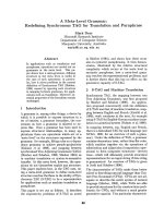
medium and large contacts). Table 2 shows how to
depict two interacting polypeptide chains by means of a
macromolecular pseudograph because the heterodimer
(SKEERN) contains an amino acid with a hydrogen
bond between its side-chain and its main-chain atom.
The n · nkth nonstochastic graph–theoretic elec-
tronic-contact matrix, M

k
m
, is a square and symmetric
matrix, where n is the number of amino acids in the
protein [6,28]. The coefficients
k
m
ij
are the elements of
the kth power of M
m
and are defined as:
m
ij
¼ 1if i 6¼ j and 9 e
k
2 EðG
m
Þð1Þ
=1 if i = j and the amino acid i has a hydrogen
bond between its side-chain and its main-chain atom,
= 0 otherwise.
where E(G
m
) represents the set of edges of G
m
.
The matrix M
k
m

provides the number of walks of
length k that link every pair of vertices v
i
and v
j
. For
this reason, each edge in M
1
m
represents a peptidic
bond (covalent bond) or a hydrogen bond as well as a
salt-bridge interaction (noncovalent bond) between
amino acids i and j.
On the other hand, the kth stochastic graph–theo-
retic electronic-contact matrix of G
m
,
s
M
k
m
, can be
Table 2. Representation of two interacting polypeptide chains and its associated pseudograph and macromolecular vector.
46

Ser
Lys
Glu

Glu
Arg
Asn

1
2
3
4
56
NH
2
COOH
chain 1
chain 2
2
3
4
5
6
1
Cα
Cα
Cα
Cα
Cα
Cα
NH
2
NH
2

NH
2
COOH
COOH
COOH
Macromolecular ‘pseudograph’ (G
m
) of the a-carbon
atoms (polypeptide’s backbone):
Here, we consider both the covalent interaction (peptidic bond
between amino acid shown with solid line) and the noncovalent
interaction (salt-bridge and hydrogen bond shown with dashed line)
between amino acid side-chains (R-groups) in the same polypeptidic chain
or different chains. The loop in the third position (Glu
3
) indicates a hydrogen
bond between an amino acid main chain and its side-chain
Macromolecular vector:

x
m
¼½SKEERN2R
6
In the definition of the

x
m
, as macromolecular
vector, the one-letter symbol of the amino acids
indicates the corresponding side-chain amino acid

property, e.g. z
1
-values. That is to say, if we write S,
it means z
1
(S), z
1
-values or some amino acid property,
which characterizes each side chain in the polypeptide.
Therefore, if we use the canonical bases of R
6
, the
coordinates of any vector

x
m
coincide with the
components of that macromolecular vector.
½X
m

T
¼½SKEERN
[X
m
]
T
= transposed of [X
m
] and it means the vector of the

coordinates of

x
m
in the canonical basis of R
6
(a 1 · 6 matrix)
[X
m
]: vector of coordinates of

x
m
in the canonical basis of R
6
(a 6 · 1matrix)

x
m
,

y
m
components are z
1
and z
2
-values, respectively.

x

m
¼½1:96 2:84 3:08 3:08 2:88 3:22 

y
m
¼

y
m
¼½À1:63 1:41 0:39 0:39 2:52 1:45 
S. E. Ortega-Broche et al. Predicting the stability of the Arc repressor
FEBS Journal 277 (2010) 3118–3146 ª 2010 The Authors Journal compilation ª 2010 FEBS 3121
directly obtained from M
k
m
. Here,
s
M
k
m
=[
k
sm
ij
], is a
square matrix of order n (n = number of C
a
atoms)
and the elements
k

sm
ij
are defined as:
k
sm
ij
¼
k
m
ij
k
SUM
i
¼
k
m
ij
k
d
i
ð2Þ
where,
k
m
ij
are the elements of the kth power of M
k
m
and the sum of the ith row of M
k

m
is named the k-order
vertex degree of C
a
atom i,
k
d
i
. It should be noted that
the matrix
s
M
k
m
in Eqn (2) has the property that the
sum of the elements in each row is 1. An n · n matrix
with nonnegative entries having this property is called
a ‘stochastic matrix’ [57]. Table 3 shows the zero, first
and second powers of the total nonstochastic and sto-
chastic graph–theoretic electronic-contact matrices of
macromolecular pseudograph depicted in Table 2.
Mathematical bilinear forms: a theoretical
framework
In mathematics, a bilinear form in a real vector space
is a mapping b:V Â V !<, which is linear in both
arguments [58–63]. That is, this function satisfies the
following axioms for any scalar a and any choice of
vectors

v;


w;

v
1
;

v
2
;

w
1
and

w
2
:
(1) bða

v;

wÞ¼bð

v; a

wÞ¼abð

v;


wÞ
(2) bð

v
1
þ

v
2
;

wÞ¼bð

v
1
;

wÞþbð

v
2
;

wÞ
(3) bð

v;

w
1

þ

w
2
Þ¼bð

v;

w
1
Þþbð

v;

w
2
Þ
That is, b is bilinear if it is linear in each parameter,
taken separately.
Let V be a real vector space in <
n
ðV 2<
n
Þ and con-
sider that the following vector set,

e
1
;


e
2
; ;

e
n
fg
is a
basis set of <
n
. This basis set permits us to write in
unambiguous form any vectors

x and

y of V, where
ðx
1
; x
2
; ; x
n
Þ2<
n
and ðy
1
; y
2
; ; y
n

Þ2<
n
are the
coordinates of the vectors

x and

y, respectively. That is
to say:

x ¼
X
n
i¼1
x
i

e
i
ð3Þ
and

y ¼
X
n
j¼1
y
j

e

j
ð4Þ
Subsequently,
bð

x;

yÞ¼bðx
i

e
i
; y
j

e
j
Þ¼x
i
y
j
bð

e
i
;

e
j
Þð5Þ

if we take the a
ij
as the n · n scalars bð

e
i
;

e
j
Þ. That is:
a
ij
¼ bð

e
i
;

e
j
Þ; to i ¼ 1; 2; ; n and j ¼ 1; 2; ; n ð6Þ
Then:
bð

x;

yÞ¼
X
n

i;j
a
ij
x
i
y
j
¼ X½
T
AY½¼
x
1
::: x
n
ÂÃ
a
11
::: a
jn
::: ::: :::
a
n1
::: a
nn
2
4
3
5
y
1

.
.
.
y
n
2
6
4
3
7
5
ð7Þ
As can be seen, the defined equation for b may be
written as the single matrix equation [see Eqn (7)],
where [Y] is a column vector (an n · 1 matrix) of the
coordinates of

y in a basis set of <
n
, and [X]
T
(a 1 · n
matrix) is the transpose of [X], where [X] is a column
vector (an n · 1 matrix) of the coordinates of

x in the
same basis of <
n
:
Finally, we introduce the formal definition of sym-

metric bilinear form. Let V be a real vector space and
b be a bilinear function in V · V. The bilinear function
Table 3. The zero (k = 0), first (k = 1) and second (k = 2) powers of the total nonstochastic and stochastic graph–theoretic electronic-contact
matrices of G
m
, respectively.
Order (k) Nonstochastic Stochastic
k =0
100000
010000
001000
000100
000010
000001
2
6
6
6
6
6
6
4
3
7
7
7
7
7
7
5

100000
010000
001000
000100
000010
000001
2
6
6
6
6
6
6
4
3
7
7
7
7
7
7
5
k =1
010010
101001
011000
000011
100101
010110
2

6
6
6
6
6
6
4
3
7
7
7
7
7
7
5
0
1
2
00
1
2
0
1
3
0
1
3
00
1
3

0
1
2
1
2
000
0000
1
2
1
2
1
3
00
1
3
0
1
3
0
1
3
0
1
3
1
3
0
2
6

6
6
6
6
6
6
4
3
7
7
7
7
7
7
7
5
k =2
201102
031120
112001
110211
020131
201113
2
6
6
6
6
6
6

4
3
7
7
7
7
7
7
5
1
3
0
1
6
1
6
0
1
3
0
3
7
1
7
1
7
2
7
0
1

5
1
5
2
5
00
1
5
1
6
1
6
0
1
3
1
6
1
6
0
2
7
0
1
7
3
7
1
7
1

4
0
1
8
1
8
1
8
3
8
2
6
6
6
6
6
6
6
4
3
7
7
7
7
7
7
7
5
Predicting the stability of the Arc repressor S. E. Ortega-Broche et al.
3122 FEBS Journal 277 (2010) 3118–3146 ª 2010 The Authors Journal compilation ª 2010 FEBS

b is called symmetric if bð

x;

yÞ¼bð

y;

xÞ; 8

x;

y 2 V [58–
63]. Then:
bð

x;

yÞ¼
X
n
i;j
a
ij
x
i
y
j
¼
X

n
i;j
a
ji
x
j
y
i
¼ bð

y;

xÞð8Þ
Nonstochastic and stochastic amino acid-based
bilinear indices: total (global) definition
The kth nonstochastic and stochastic bilinear indices
for a protein, b
m
k
ð

x
m
;

y
m
Þ and
s
b

m
k
ð

x
m
;

y
m
Þ, are com-
puted from these kth nonstochastic and stochastic
graph–theoretic electronic-contact matrix, M
k
m
and
s
M
k
m
as shown in Eqns (9) and (10), respectively:
b
mk
ð

x
m
;

y

m
Þ¼
X
n
i¼1
X
n
j¼1
k
m
ij
x
i
m
y
j
m
ð9Þ
s
b
mk
ð

x
m
;

y
m
Þ¼

X
n
i¼1
X
n
j¼1
k
sm
ij
x
i
m
y
j
m
ð10Þ
where n is the number of amino acids (C
a
atom) in the
protein, and x
1
m
; ; x
n
m
and y
1
m
; ; y
n

m
are the coordi-
nates or components of the macromolecular vectors

x
m
and

y
m
in a canonical basis set of <
n
:
The defined Eqns (9) and (10) for b
m
k
ð

x
m
;

y
m
Þ and
s
b
m
k
ð


x
m
;

y
m
Þ may be also written as the single matrix
equations:
b
m
k
ð

x
m
;

y
m
Þ¼½X
m

T
M
k
m
½Y
m
ð11Þ

s
b
m
k
ð

x
m
;

y
m
Þ¼½X
m

Ts
M
k
m
½Y
m
ð12Þ
where [Y
m
] is a column vector (an n · 1 matrix) of the
coordinates of

y
m
in the canonical basis set of <

n
, and
[X
m
]
T
is the transpose of [X
m
], where [X
m
] is a column
vector (an n · 1 matrix) of the coordinates of

x
m
in the
canonical basis of <
n
: Therefore, if we use the canoni-
cal basis set, the coordinates [(x
1
m
, , x
n
m
) and (y
1
m
, ,
y

n
m
)] of any macromolecular vectors (

x
m
and

y
m
) coin-
cide with the components of those vectors [(x
m1
, ,
x
mn
) and (y
m1
, , y
mn
)]. For that reason, those coordi-
nates can be considered as weights (R-group in C
a
atom, that is to say ‘amino acid labels’) of the vertices
of G
m
, as a result of the fact that components of the
molecular vectors are values of some amino acid
property that characterizes each kind of R-chain in the
protein. The calculation of the three first values of

bilinear indices for the example protein (Tables 2 and
3) is shown in Table 4.
It should be noted that nonstochastic and stochastic
bilinear indices are symmetric and nonsymmetric bilin-
ear forms, respectively. Therefore, if, in the following
weighting scheme, W and Z are used as amino acid
weights to compute the protein bilinear indices, two dif-
ferent sets of stochastic bilinear indices,
WÀZs
b
m
k
ð

x
m
;

y
m
Þ
and
ZÀWs
b
m
k
ð

x
m

;

y
m
Þ [because

x
mW
À

y
mZ
6¼

x
mZ
À

y
mW
]
can be obtained, and only one group of nonstochastic
bilinear i ndices
WÀZ
b
m
k
ð

x

m
;

y
m
Þ¼
ZÀW
b
m
k
ð

x
m
;

y
m
Þ because,
in this case,

x
mW
À

y
mZ
¼

x

mZ
À

y
mW
can be calculated.
Nonstochastic and stochastic local bilinear
indices: definition of amino acid, amino
acid-type and peptide fragment bilinear indices
In the last decade, Randic
´
[64] proposed a list of desir-
able attributes for a molecular descriptor. Therefore,
this list can be considered as a methodological guide
for the development of new topological indices. One of
the most important criteria is the possibility of defining
the descriptors locally. This attribute refers to the
fact that the index could be calculated for the molecule
(protein) as a whole but also over certain fragments of
the structure itself.
Therefore, in addition to total bilinear indices com-
puted for the whole protein, a local-fragment (peptide
fragment) formalism can be developed. These descrip-
tors are termed local nonstochastic and stochastic
bilinear indices: b
mk
L
ð

x

m
;

y
m
Þ and
s
b
mk
L
ð

x
m
;

y
m
Þ, respec-
tively. The definition of these descriptors is:
b
mk
L
ð

x
m
;

y

m
Þ¼
X
n
i¼1
X
n
j¼1
k
m
ij
L
x
i
m
y
j
m
ð13Þ
s
b
mk
L
ð

x
m
;

y

m
Þ¼
X
n
i¼1
X
n
j¼1
k
sm
ij
L
x
i
m
y
j
m
ð14Þ
where
k
m
ijL
[
k
sm
ijL
] is the kth element of the row ‘i’
and column ‘j’ of the local matrix M
k

mL
½
s
M
k
mL
. This
matrix is extracted from the M
k
m
½
s
M
k
m
 matrix and
contains information referring to the vertices of the
specific protein fragments (F
r
) and also to the molecu-
lar environment in step k. The matrix M
k
mL
½
s
M
k
mL
 with
elements

k
m
ijL
[
k
sm
ijL
] is defined as (Table 5):
k
m
ijL
[
k
sm
ijL
]=
k
m
ij
[
k
sm
ijL
] if both v
i
and v
j
are
vertices (amino acid) contained within the F
r

=1⁄ 2
k
m
ij
[
k
sm
ijL
]ifv
i
or v
j
are vertices contained
within F
r
but not both
¼ 0 otherwise ð15Þ
These local analogues can also be expressed in
matrix form by the expressions:
b
mk
L
ð

x
m
;

y
m

Þ¼½X
m

T
M
k
mL
½Y
m
ð16Þ
s
b
m
k
ð

x
m
;

y
m
Þ¼½X
m

Ts
M
k
mL
½Y

m
ð17Þ
S. E. Ortega-Broche et al. Predicting the stability of the Arc repressor
FEBS Journal 277 (2010) 3118–3146 ª 2010 The Authors Journal compilation ª 2010 FEBS 3123
It should be noted that the scheme above follows
the spirit of a Mulliken population analysis [65]. It
should be also noted that for every partitioning of a
protein into Z macromolecular fragments, there will be
Z local macromolecular fragment matrices. In this
case, if a protein is partitioned into Z molecular frag-
ments, the matrix M
k
m
½
s
M
k
m
 can be correspondingly
partitioned into Z local matrices M
k
mL
½
s
M
k
mL
, L =1,
, Z, and the kth power of matrix M
k

m
½
s
M
k
m
 is exactly
the sum of the kth power of the local Z matrices. In
this way, the total nonstochastic and stochastic bilinear
indices are the sum of the nonstochastic and stochastic
bilinear indices, respectively, of the Z macromolecular
fragments:
b
m
ð

x
m
;

y
m
Þ¼
X
Z
L¼1
b
mkL
ð


x
m
;

y
m
Þð18Þ
s
b
m
ð

x
m
;

y
m
Þ¼
X
Z
L¼1
s
b
mkL
ð

x
m
;


y
m
Þð19Þ
In addition, the amino acid-type bilinear indices can
also be calculated. Amino acid and amino acid-type
bilinear indices are specific cases of local protein bilin-
ear indices. In this sense, the kth amino acid-bilinear
indices are calculated by summing the kth amino acid
bilinear indices of all amino acids of the same amino
Table 4. Values of nonstochastic and stochastic total bilinear indices for two interacting peptides (SKEERN) used as example above (see
also Tables 2 and 3).
Nonstochastic total bilinear indices
b
m0
¼
P
n
i¼1
P
n
j¼1
0
m
ij
x
i
m
y
j

m
¼½X
m

T
M
0
m
½Y
m
¼½1:96 2:84 3:08 3:08 2:88 3:22 
100000
010000
001000
000100
000010
000001
2
6
6
6
6
6
6
4
3
7
7
7
7

7
7
5
À1:63
1:41
0:39
0:39
2:52
1:45
2
6
6
6
6
6
6
4
3
7
7
7
7
7
7
5
¼ 15:14
b
m1
¼
P

n
i¼1
P
n
j¼1
1
m
ij
x
i
m
y
j
m
¼½X
m

T
M
1
m
½Y
m
¼½1:96 2:84 3:08 3:08 2:88 3:22
010010
101001
011000
000011
100101
010110

2
6
6
6
6
6
6
4
3
7
7
7
7
7
7
5
À1:63
1:41
0:39
0:39
2:52
1:45
2
6
6
6
6
6
6
4

3
7
7
7
7
7
7
5
¼ 40:59
b
m2
¼
P
n
i¼1
P
n
j¼1
2
m
ij
x
i
m
y
j
m
¼½X
m


T
M
2
m
½Y
m
¼½1:96 2:84 3:08 3:08 2:88 3:22 
201102
031120
112001
110211
020131
201113
2
6
6
6
6
6
6
4
3
7
7
7
7
7
7
5
À1:63

1:41
0:39
0:39
2:52
1:45
2
6
6
6
6
6
6
4
3
7
7
7
7
7
7
5
¼ 98:84
Stochastic total bilinear indices
s
b
m0
¼
P
n
i¼1

P
n
j¼1
0
sm
ij
x
i
m
y
j
m
¼½X
m

T
s
M
0
m
½Y
m
¼½1:96 2:84 3:08 3:08 2:88 3:22 
100000
010000
001000
000100
000010
000001
2

6
6
6
6
6
6
4
3
7
7
7
7
7
7
5
À1:63
1:41
0:39
0:39
2:52
1:45
2
6
6
6
6
6
6
4
3

7
7
7
7
7
7
5
¼ 15:14
s
b
m1
¼
P
n
i¼1
P
n
j¼1
1
sm
ij
x
i
m
y
j
m
¼½X
m


T
s
M
1
m
½Y
m
¼½1:96 2:84 3:08 3:08 2:88 3:22 
0
1
2
00
1
2
0
1
3
0
1
3
00
1
3
0
1
2
1
2
000
0000

1
2
1
2
1
3
00
1
3
0
1
3
0
1
3
0
1
3
1
3
0
2
6
6
6
6
6
6
6
6

4
3
7
7
7
7
7
7
7
7
5
À1:63
1:41
0:39
0:39
2:52
1:45
2
6
6
6
6
6
6
6
6
4
3
7
7

7
7
7
7
7
7
5
¼ 17:77
s
b
m2
¼
P
n
i¼1
P
n
j¼1
2
sm
ij
x
i
m
y
j
m
¼½X
m


T
s
M
2
m
½Y
m
¼½1:96 2:84 3:08 3:08 2:88 3:22 
1
3
0
1
6
1
6
0
1
3
0
3
7
1
7
1
7
2
7
0
1
5

1
5
2
5
00
1
5
1
6
1
6
0
1
3
1
6
1
6
0
2
7
0
1
7
3
7
1
7
1
4

0
1
8
1
8
1
8
3
8
2
6
6
6
6
6
6
6
6
4
3
7
7
7
7
7
7
7
7
5
À1:63

1:41
0:39
0:39
2:52
1:45
2
6
6
6
6
6
6
6
6
4
3
7
7
7
7
7
7
7
7
5
¼ 14:57
Predicting the stability of the Arc repressor S. E. Ortega-Broche et al.
3124 FEBS Journal 277 (2010) 3118–3146 ª 2010 The Authors Journal compilation ª 2010 FEBS
Table 5. The zero (k = 0), first (k = 1) and second (k = 2) powers of the local nonstochastic and stochastic graph–theoretic electronic-
contact matrices of G

m
, respectively.
The zero, first and second powers of the local (amino acid) nonstochastic matrices
M
0
ðG
m
; SÞ¼
100000
000000
000000
000000
000000
000000
2
6
6
6
6
6
6
4
3
7
7
7
7
7
7
5

M
1
ðG
m
; SÞ¼
0
1
2
00
1
2
0
1
2
00000
000000
000000
1
2
00000
000000
2
6
6
6
6
6
6
4
3

7
7
7
7
7
7
5
M
2
ðG
m
; SÞ¼
20
1
2
1
2
01
000000
1
2
00000
1
2
00000
000000
100000
2
6
6

6
6
6
6
4
3
7
7
7
7
7
7
5
M
0
ðG
m
; KÞ¼
000000
010000
000000
000000
000000
000000
2
6
6
6
6
6

6
4
3
7
7
7
7
7
7
5
M
1
ðG
m
; KÞ¼
1
1
2
0000
1
2
0
1
2
00
1
2
0
1
2

0000
000000
000000
0
1
2
0000
2
6
6
6
6
6
6
4
3
7
7
7
7
7
7
5
M
2
ðG
m
; K Þ¼
000000
03

1
2
1
2
10
0
1
2
0000
0
1
2
0000
010000
000000
2
6
6
6
6
6
6
4
3
7
7
7
7
7
7

5
M
0
ðG
m
; EÞ¼
000000
000000
001000
000000
000000
000000
2
6
6
6
6
6
6
4
3
7
7
7
7
7
7
5
M
1

ðG
m
; EÞ¼
000000
00
1
2
000
0
1
2
1000
000000
000000
000000
2
6
6
6
6
6
6
4
3
7
7
7
7
7
7

5
M
2
ðG
m
; EÞ¼
00
1
2
000
00
1
2
000
1
2
1
2
200
1
2
000000
000000
00
1
2
000
2
6
6

6
6
6
6
4
3
7
7
7
7
7
7
5
M
0
ðG
m
; EÞ¼
000000
000000
000000
000100
000000
000000
2
6
6
6
6
6

6
4
3
7
7
7
7
7
7
5
M
1
ðG
m
; EÞ¼
000000
000000
000000
0000
1
2
1
2
000
1
2
00
000
1
2

00
2
6
6
6
6
6
6
4
3
7
7
7
7
7
7
5
M
2
ðG
m
; EÞ¼
000
1
2
00
000
1
2
00

000000
1
2
1
2
02
1
2
1
2
000
1
2
00
000
1
2
00
2
6
6
6
6
6
6
4
3
7
7
7

7
7
7
5
M
0
ðG
m
; RÞ¼
000000
000000
000000
000000
000010
000000
2
6
6
6
6
6
6
4
3
7
7
7
7
7
7

5
M
1
ðG
m
; RÞ¼
0000
1
2
0
000000
000000
0000
1
2
0
1
2
00
1
2
0
1
2
0000
1
2
0
2
6

6
6
6
6
6
4
3
7
7
7
7
7
7
5
M
2
ðG
m
; RÞ¼
000000
000010
000000
0000
1
2
0
010
1
2
3

1
2
0000
1
2
0
2
6
6
6
6
6
6
4
3
7
7
7
7
7
7
5
M
0
ðG
m
; NÞ¼
000000
000000
000000

000000
000000
000001
2
6
6
6
6
6
6
4
3
7
7
7
7
7
7
5
M
1
ðG
m
; NÞ¼
000000
00000
1
2
000000
00000

1
2
00000
1
2
0
1
2
0
1
2
1
2
0
2
6
6
6
6
6
6
4
3
7
7
7
7
7
7
5

M
0
ðG
m
; NÞ¼
000001
000000
00000
1
2
00000
1
2
00000
1
2
10
1
2
1
2
1
2
3
2
6
6
6
6
6

6
6
4
3
7
7
7
7
7
7
7
5
The zero, first and second powers of the local (amino acid) stochastic matrices
M
0
ðG
m
; SÞ¼
100000
000000
000000
000000
000000
000000
2
6
6
6
6
6

6
4
3
7
7
7
7
7
7
5
M
1
ðG
m
; SÞ¼
0
1
4
00
1
4
0
1
6
00000
000000
000000
1
6
00000

000000
2
6
6
6
6
6
6
4
3
7
7
7
7
7
7
5
M
2
ðG
m
; SÞ¼
1
3
0
1
12
1
12
0

1
6
1
6
00000
1
10
00000
1
12
00000
1
8
00000
000000
2
6
6
6
6
6
6
6
6
4
3
7
7
7
7

7
7
7
7
5
M
0
ðG
m
; KÞ¼
000000
010000
000000
000000
000000
000000
2
6
6
6
6
6
6
4
3
7
7
7
7
7

7
5
M
1
ðG
m
; KÞ¼
0
1
4
0000
1
6
0
1
6
00
1
6
0
1
4
0000
000000
000000
0
1
6
0000
2

6
6
6
6
6
6
4
3
7
7
7
7
7
7
5
M
2
ðG
m
; K Þ¼
000000
0
3
7
1
14
1
14
1
7

0
0
1
10
0000
0
1
12
0000
0
1
7
0000
000000
2
6
6
6
6
6
6
6
6
4
3
7
7
7
7
7

7
7
7
5
M
0
ðG
m
; EÞ¼
000000
000000
001000
000000
000000
000000
2
6
6
6
6
6
6
4
3
7
7
7
7
7
7

5
M
1
ðG
m
; EÞ¼
000000
00
1
6
000
0
1
4
1
2
000
000000
000000
000000
2
6
6
6
6
6
6
4
3
7

7
7
7
7
7
5
M
2
ðG
m
; EÞ¼
00
1
12
000
00
1
14
000
1
10
1
10
2
5
00
1
10
000000
000000

00
1
16
000
2
6
6
6
6
6
6
6
6
4
3
7
7
7
7
7
7
7
7
5
S. E. Ortega-Broche et al. Predicting the stability of the Arc repressor
FEBS Journal 277 (2010) 3118–3146 ª 2010 The Authors Journal compilation ª 2010 FEBS 3125
acid type in the protein. In the amino acid-type bilin-
ear indices formalism, each amino acid in the molecule
is classified into an amino acid-type (fragment), such
as apolar, polar uncharged, polar charged, positive

charged, negative charged, aromatic, and so on. For
all data sets, including those with a common molecular
scaffold, as well as those with very diverse structure,
the kth amino acid-type bilinear indices provide
important information. The calculation of the three
first values of local (amino acid) bilinear indices for
the example protein (Tables 2 and 3) is shown in
Table 6.
Any local protein bilinear index has a particular
meaning, especially for the first values of k, where the
information about the structure of the fragment F
R
is
contained. Higher values of k relate to the environ-
ment information of the fragment F
R
considered
within the macromolecular pseudograph.
In any case, a complete series of indices performs a
specific characterization of the chemical structure.
The generalization of the matrices and descriptors to
‘superior analogues’ is necessary for the evaluation of
situations where only one descriptor is unable to
allow good structural characterization [64,66]. The
local macromolecular indices can also be used
together with the total ones as variables for quantita-
tive structure–activity relationship (QSAR) ⁄ quantita-
tive structure–property relationship (QSPR) modelling
of properties or activities that depend more on a
region or a fragment than on the macromolecule as a

whole.
Data preparation
Computation of protein bilinear indices
The calculation of total and local macromolecular
bilinear indices for any peptide or protein was
Table 5. (Continued).
M
0
ðG
m
; EÞ¼
000000
000000
000000
000100
000000
000000
2
6
6
6
6
6
6
4
3
7
7
7
7

7
7
5
M
1
ðG
m
; EÞ¼
000000
000000
000000
0000
1
4
1
4
000
1
6
00
000
1
6
00
2
6
6
6
6
6

6
4
3
7
7
7
7
7
7
5
M
2
ðG
m
; EÞ¼
000
1
12
00
000
1
14
00
000000
1
12
1
12
0
1

3
1
12
1
12
000
1
14
00
000
1
16
00
2
6
6
6
6
6
6
6
6
4
3
7
7
7
7
7
7

7
7
5
M
0
ðG
m
; RÞ¼
000000
000000
000000
000000
000010
000000
2
6
6
6
6
6
6
4
3
7
7
7
7
7
7
5

M
1
ðG
m
; RÞ¼
0000
1
14
0
000000
00000 0
0000
1
14
0
1
6
00
1
6
0
1
6
0000
1
6
0
2
6
6

6
6
6
6
4
3
7
7
7
7
7
7
5
M
2
ðG
m
; RÞ¼
000 0 0 0
000 0
1
7
0
000 0 0 0
000 0
1
12
0
0
1

7
0
1
14
3
7
1
14
000 0
1
16
0
2
6
6
6
6
6
6
6
6
4
3
7
7
7
7
7
7
7

7
5
M
0
ðG
m
; NÞ¼
000000
000000
000000
000000
000000
000001
2
6
6
6
6
6
6
4
3
7
7
7
7
7
7
5
M

1
ðG
m
; NÞ¼
000000
00000
1
6
000000
00000
1
4
00000
1
6
0
1
6
0
1
6
1
6
0
2
6
6
6
6
6

6
4
3
7
7
7
7
7
7
5
M
2
ðG
m
; NÞ¼
000 0 0
1
6
000000
000 0 0
1
10
000 0 0
1
12
000 0 0
1
14
1
8

0
1
16
1
16
1
16
3
8
2
6
6
6
6
6
6
6
6
4
3
7
7
7
7
7
7
7
7
5
Table 6. Values of amino acid-based (local) bilinear indices for the

heterodimer SKEERN.
Amino acid
Local nonstochastic bilinear indices
b
0L
(

x
m
,

y
m
) b
1L
(

x
m
,

y
m
) b
2L
(

x
m
,


y
m
)
Ser (S) )3.1948 )0.8104 )13.0522
Lys (K) 4.0044 6.1215 28.6812
Glu (E) 1.2012 3.9264 5.8605
Glu (E) 1.2012 7.3033 10.3029
Arg (R) 7.2576 10.71 43.578
Asn (N) 4.669 13.3352 23.4674
Heterodimer
(SKEERN)
15.1386 40.586 98.8378
Amino acid
Local stochastic bilinear indices
s
b
0L
ð

x
m
;

y
m
Þ
s
b
1L

,ð

x
m
;

y
m
Þ
s
b
2L
ð

x
m
;

y
m
Þ
Ser (S) )3.1948 0.37176667 )2.04034833
Lys (K) 4.0044 2.6327 4.27309429
Glu (E) 1.2012 1.8709 1.08062179
Glu (E) 1.2012 3.4534 1.66443036
Arg (R) 7.2576 4.6284 6.24537857
Asn (N) 4.669 4.81723333 3.34964405
Heterodimer
(SKEERN)
15.1386 17.7744 14.5728207

Predicting the stability of the Arc repressor S. E. Ortega-Broche et al.
3126 FEBS Journal 277 (2010) 3118–3146 ª 2010 The Authors Journal compilation ª 2010 FEBS
implemented in tomocomd-camps software [67]. The
main steps for the application of this method in
QSAR ⁄ QSPR can be briefly summarized:
(1) Draw the macromolecular pseudographs for each
protein of the data set, using the software’s drawing
mode. This procedure is carried out by selection of the
active amino acid symbol belonging to the ‘natural’
amino acid code. Here, we consider covalent (peptidic
bond) and noncovalent [hydrogen bond and other elec-
trostatic interaction (within a chain as well as between
chains)] interaction. Afterwards, we draw the mutants
by changing an amino acid for alanine and considering
that this change only affects the possibility of this
region of the protein to form a polar interaction
(because we suppressed the hydrogen interaction if the
former amino acid had it).
(2) Use appropriated amino acid weights to differenti-
ate the side-chain of each amino acid. In the present
study, we used some descriptors for the natural amino
acid as the amino acid property: the three z-values
[48], Kyte–Doolittle’s hydrophobicity scale [50], ISA
and ECI [49].
(3) Compute the nonstochastic and stochastic protein
bilinear indices. They can be performed in the software
calculation mode, where it is possible to select the
side-chain properties and the family descriptor previ-
ously to calculate the bio-macromolecular indices. This
software generates a table in which the rows and

columns correspond to the compounds and the
b
mk
ð

x
m
;

y
m
Þ,respectively.
(4) Find a QSPR ⁄ QSAR equation by using statistical
techniques, such as multilinear regression analysis,
neural networks, linear discrimination analysis (LDA),
and so on. That is to say, we can find a quantitative
relationship between a property P and the b
mk
ð

x
m
;

y
m
Þ
having, for example, the appearance:
P ¼ a
0

b
m0
ðx
m
; y
m
Þþa
1
b
m1
ðx
m
; y
m
Þþa
2
b
m2
ðx
m
; y
m
Þ
þ ÁÁÁþa
k
b
mk
ðx
m
; y

m
Þþc ð20Þ
where P is the measurement of the property,
b
mk
ð

x
m
;

y
m
Þ½or b
mkL
ð

x
m
;

y
m
Þ is the kth total [or local]
macromolecular nonstochastic bilinear indices, and
the a
k
are the coefficients obtained by the statistical
analysis.
(5) Test the robustness and predictive power of the

QSPR ⁄ QSAR equation by using internal and external
cross-validation techniques.
(6) Develop a structural interpretation of the obtained
QSAR ⁄ QSPR model using macromolecular bilinear
indices as molecular descriptors.
Database
Arc is a homodimer in which each monomer inter-
twines with the other to form a single, globular domain
with a well-defined core. Several side-chain hydrogen
bond and salt-bridge interactions are involved in the
Arc crystal structure. An exhaustive representation of
these interactions are provided in detail elsewhere [32].
Nevertheless, an overview of these electrostatic interac-
tions in Arc repressor structure will be given. Hydro-
gen bond interactions take place [32]:
(1) Between a side-chain in the same subunit (N29-
E36) and between side-chains in different subunits
(R40-S44).
(2) Between a side-chain and main-chain atom
intersubunit (W14-N34, N34-R13) and between a
side-chain and main-chain atom intrasubunits (E17-
E17, S32-S35, S44-R40).
On the other hand, salt-bridge interactions take
place [32]:
(3) Between a side-chain in the same subunit (R16-
D20, D20-R23, R31-E36, E36-R40, E43-K46, E43-
K47) and between side-chains in different subunits
(E28-R50, R40-E48).
The data of Arc repressor mutants were taken from
the literature. In the present study, alanine substitu-

tions were constructed at each of the 51 non-alanine
positions in the wild-type Arc sequence. To avoid
intracellular proteolysis and purification difficulties,
the alanine substitution mutant was constructed in
backgrounds containing the carboxy-terminal exten-
sions (His)
6
(designated st6) or (His)
6
-Lys-Asn-Gln-
His-Glu (designated st11) [68,69]. These tail sequences
allow affinity purification, reduce degradation and
cause no significant changes in protein stability [70].
Milla et al. [32] subjected each purified mutant of
Arc to thermal and urea denaturation experiments. The
stability of the proteins was checked by melting temper-
ature (t
m
). The values of t
m
for 53 Arc homodimers
reported by these authors are given in Tables 7 and 8.
In equilibrium and kinetic unfolding–refolding stud-
ies, only native Arc dimers and denatured monomers
are significantly populated. Thus, folding and dimer-
ization are concerted processes [32,71,72]. For this
reason, it is important to note that t
m
refers to the
unfolding of the Arc homodimer. Accordingly, the fact

that each single mutation changes two side-chains in
the Arc dimer one must take into consideration, with
stability effects being approximately twice those
observed for monomeric proteins. Moreover, changes
in stability may arise as a result of mutation disrupts
of a native interaction, when the native structure of
S. E. Ortega-Broche et al. Predicting the stability of the Arc repressor
FEBS Journal 277 (2010) 3118–3146 ª 2010 The Authors Journal compilation ª 2010 FEBS 3127
the mutant undergoes relaxation, or because of a
change in the properties of the denatured mutant pro-
tein [32,73–76].
Classification- and regression-based
models for predicting Arc mutant’s
stabilities
Statistical methodologies
LDA, linear multiple regression (LMR) and the non-
linear estimation analysis, piecewise linear regression
(PLR), were used to obtain mathematical models.
These statistical analyses were carried out using the
statistica software package [77]. Forward stepwise
was fixed as the strategy for variable selection in the
case of LDA and LMR analysis. The tolerance param-
eter (i.e. the proportion of variance that is unique to
the respective variable) used was the default value for
minimum acceptable tolerance, which is 0.01.
LDA is used to generate a classifier function on the
basis of the simplicity of the method [78]. To test the
quality of the discriminant functions derived, we used
the Wilks’ k and the Mahalanobis distance. The Wilks’
k statistic for overall discrimination can take values in

the range of 0 (perfect discrimination) to 1 (no dis-
crimination). The Mahalanobis distance indicates the
separation of the respective groups. It shows whether
the model possesses an appropriate discriminatory
power for differentiating between the two respective
groups. The classification of cases was performed by
means of a posteriori classification probability, which
is the probability that the respective case belongs to a
particular group [i.e. mutants with near wild-type sta-
bility (H) or mutants with reduced stability (P)]. In
developing this classification function, the values of 1
and )1 were assigned to H and P mutants (Table 9).
The quality of the LDA model was also determined by
examining the percentage of good classification and
the proportion between the cases and variables in the
equation.
Linear and other nonlinear regression models were
obtained using LMR and PLR as statistical tech-
niques, respectively. To evaluate the fitted accuracy of
Table 7. Experimental and calculated values of melting temperature (t
m
) obtained by using Eqn (27).
Mutant Obs.
a
Cal.
b
Res.
c
Res
CV

d
Mutant Obs.
a
Cal.
b
Res.
c
Res
CV
d
1 PA8-st6 74.1 Outlier 25 EA43-st6 56.1 52.0 )4.06 )4.62
2 SA35-st6 63.4 60.6 )2.85 )3.59 26 EA28-st11 55.7 57.9 2.15 3.00
3 NA34-st11 63.0 55.6 )7.36 )8.48 27 MA7-st6 55.5 53.7 )1.84 )2.14
4 NA11-st6* 62.1 58.6 )3.50 – 28 DA20-st6 55.3 59.5 4.20 5.47
5 QA39-st11 61.4 57.3 )4.13 )4.57 29 IA51-st11 50.9 50.4 )0.50 ) 0.72
6 GA52-st11 60.9 64.0 3.05 4.19 30 GA49-st11* 48.7 52.8 4.12 –
7 KA6-st6* 59.6 62.8 3.23 – 31 LA19-st6 48.3 46.6 V1.69 )2.14
8 RA16-st6 59.5 57.7 )1.83 )2.24 32 GA30-st11 47.9 46.7 )1.21 )1.65
9 VA25-st6 59.3 56.5 )2.82 )3.09 33 RA50-st11 47.9 45.8 )2.06 )2.75
10 MA4-st6 59.2 60.5 1.32 1.78 34 KA47-st11 47.2 48.3 1.10 2.04
11 Arc-st6* 59.0 61.2 2.19 – 35 PA15-st11* 46.6 48.1 1.48 )
12 EA27-st6 58.8 59.5 0.68 0.75 36 SA44-st11 46.3 42.6 )3.69 )4.61
13 KA2-st6 58.7 585 )0.19 )0.24 37 NA29-st11 45.3 46.4 1.14 1.36
14 QA9-st6 58.4 60.3 1.92 2.29 38 VA33-st11 44.1 48.7 4.56 5.04
15 GA3-st6 58.1 62.1 4.02 4.47 39 EA48-st11 43.2 47.2 3.95 4.58
16 MA1-st6* 58.0 54.8 )3.16 ) 40 LA12-st11 42.3 39.8 )2.49 )3.12
17 Arc-st11 57.9 54.3 )3.65 )4.11 41 FA10-st6* 40.6 46.7 6.08 )
18 SA5-st6* 57.5 61.7 4.23 – 42 LA21-st11 39.6 39.2 )0.36 )0.45
19 RA13-st6 57.3 55.8 )1.52 )2.09 43 RA31-st11 37.1 41.2 4.12 4.60
20 KA46-st11 57.1 54.8 )2.29 )2.67 44 MA42-st11 35.6 42.1 6.47 7.41

21 EA17-st6 57.0 63.5 6,5 7.48 45 SA32-st11 33.5 Outlier
22 VA18-st6 56.9 53.0 )
3.93 )4.47 46 YA38-st11 33.0 38.1 5.08 6.51
23 RA23-st11 56.7 49.2 )7.55 )7.96 47 WA14-st11* 31.5 23.8 )7.68 –
24 KA24-st11 56.3 60.3 4.01 4.67 48 RA40-st11 31.2 32.9 1.73 3.79
a
Experimental melting temperature (t
m
)in°C [32]: proteins are arranged in order of decreasing t
m
; mutants 49–53 (VA22-st11, EA36-st11,
IA37-st11, VA41-st11 and FA45-st11) were not included in this QSAR study as a result of non-accurate values of t
m
(< 20 °C), which are not
useful for regression analysis. The st6 and st11 refer to C-terminal sequences of the mutant proteins [32].
b
Calculated t
m
values by using
Eqn (27).
c
Residual: t
m
(Obs.) ) t
m
(Cal.).
d
Residual by LOO cross-validation procedures (deleted residual). *Cases that were selected
randomly for use in the external validation.
Predicting the stability of the Arc repressor S. E. Ortega-Broche et al.

3128 FEBS Journal 277 (2010) 3118–3146 ª 2010 The Authors Journal compilation ª 2010 FEBS
these models, we examined the determination coeffi-
cient (R
2
), Fisher ratio’s P-level [P(F)] and the
standard error in calculation (SDEC). Leave-one out
(LOO), bootstrapping (BOOT) and Y-scrambling were
the procedures used for the assessment of the internal
validity of models obtained by multivariate regression
methods. Specifically, the cross-validated determination
coefficient calculated in LOO (q
2
LOO
) and BOOT
(q
2
BOOT
) strategies were used to evaluate the robustness
and stability of the linear regression equations,
together with the standard error in prediction (SDEP);
the parameters a(R
2
) and a(q
2
) estimated in a Y-ran-
domization experiment were also calculated to test the
absence of chance correlation [79].
Recently, many studies have used q
2
LOO

to assess
the predictive power and have considered high q
2
LOO
values (e.g. q
2
LOO
> 0.5) as an indicator (or even as
the ultimate proof) of the high-predictive power of a
QSAR model [80]. However, Golbraikh and Tropsha
[81] demonstrated that a high value of q
2
LOO
appears
to be a necessary but not sufficient condition for the
model to have a high predictive power. These authors
stated that the predictability of a QSAR model can
only be estimated using an external set of compounds
that was not used for building the model [81,82].
Therefore, to assess the predictive power of the clas-
sification and regression models developed in the
present study, external (test) sets were used. The sta-
tistical parameters and criteria used for the assess-
ment of the predictive ability of the multivariate
regression models were:
q
2
ext
¼ 1 À
P

n
ext
i¼1
y
obs
i
À y
pred
i

P
n
ext
i
y
obs
i
À y
train
i
ÀÁ
ð21Þ
R
ext
> 0:77 or R
2
ext
> 0:6 ð22Þ
R
2

ext
À R
2
0;ext
R
2
ext
< 0:1 or
R
2
ext
À R
02
0;ext
R
2
ext
< 0:1 ð23Þ
0:85 k 1:15 or 0:85 k
0
1:15 ð24Þ
where q
2
ext
is external determination coefficient indicat-
ing predictive ability on the test by the model; y
obs
i
Table 8. Experimental and calculated values of melting temperature (t
m

) obtained by using Eqn (28).
Mutant Obs.
a
Cal.
b
Res.
c
Res
CV
d
Mutant Obs.
a
Cal.
b
Res.
c
Res
CV
d
1 PA8-st6 74.1 Outlier 25 EA43-st6 56.1 55.6 )0.53 )0.60
2 SA35-st6 63.4 60.6 )3.13 )3.53 26 EA28-st11 55.7 56.9 1.21 2.10
3 NA34-st11 63.0 55.6 )6.43 )9.44 27 MA7-st6 55.5 57.2 1.72 1.96
4 NA11-st6* 62.1 53.5 )8.58 – 28 DA20-st6 55.3 60.2 4.90 7.20
5 QA39-st11 61.4 57.3 )6.45 )7.11 29 IA51-st11 50.9 51.6 0.71 0.81
6 GA52-st11 60.9 64.0 0.66 0.82 30 GA49-st11* 48.7 58.7 10.7 –
7 KA6-st6* 59.6 59.2 )0.36 – 31 LA19-st6 48.3 48.1 )0.23 )0.27
8 RA16-st6 59.5 57.7 2.40 3.11 32 GA30-st11 47.9 45.8 )2.12 )2.68
9 VA25-st6 59.3 56.5 )1.98 )2.25 33 RA50-st11 47.9 52.1 4.16 6.34
10 MA4-st6 59.2 60.5 )7.94 )9.68 34 KA47-st11 47.2 53.4 6.15 6.75
11 Arc-st6* 59.0 58.9 )0.14 – 35 PA15-st11* 46.6 54.1 7.48 –

12 EA27-st6 58.8 59.5 0.11 0.13 36 SA44-st11 46.3 47.0 0.74 0.78
13 KA2-st6 58.7 58.5 )4.33 )5.73 37 NA29-st11 45.3 42.6 )2.66 )3.06
14 QA9-st6 58.4 60.3 2.12 2.79 38 VA33-st11 44.1 48.9 4.81 5.27
15 GA3-st6 58.1 62.1 1.40 1.57 39 EA48-st11 43.2 47.7 4.52 5.30
16 MA1-st6* 58.0 59.7 1.76 – 40 LA12-st11 42.3 39.5 )2.79 )5.84
17 Arc-st11 57.9 54.3 )5.09 )6.16 41 FA10-st6* 40.6 45.3 4.74 –
18 SA5-st6* 57.5 56.5 )0.96 – 42 LA21-st11 39.6 41.1 1.46 1.77
19 RA13-st6 57.3 55.8 3.66 4.59 43 RA31-st11 37.1 36.2 )0.91 )1.23
20 KA46-st11 57.1 54.8 )2.72 )2.93 44 MA42-st11 35.6 41.9 6.26 7.14
21 EA17-st6 57.0 63.5 2.00 2.48 45 SA32-st11 33.5 Outlier
22 VA18-st6 56.9 53.0 )1.57 )1.72 46 YA38-st11 33.0 34.5 1.49 1.89
23 RA23-st11 56.7 49.2 )5.61 )6.76 47 WA14-st11* 31.5 40.0 8.49 –
24 KA24-st11 56.3 60.3 2.50 3.17 48 RA40-st11 31.2 32.7 1.53 2.13
a
Experimental melting temperature (t
m
)in°C [32]: proteins are arranged in order of decreasing t
m
; mutants 49–53 (VA22-st11, EA36-st11,
IA37-st11, VA41-st11 and FA45-st11) were not included in this QSAR study as a result of non-accurate values of t
m
(< 20 °C), which are not
useful for regression analysis. The st6 and st11 refer to C-terminal sequences of the mutant proteins [32].
b
Calculated t
m
values by using
Eqn (28).
c
Residual: t

m
(Obs.) ) t
m
(Cal.).
d
Residual by LOO cross-validation procedures (deleted residual). *Cases that were selected ran-
domly for use in the external validation.
S. E. Ortega-Broche et al. Predicting the stability of the Arc repressor
FEBS Journal 277 (2010) 3118–3146 ª 2010 The Authors Journal compilation ª 2010 FEBS 3129
denotes the observed properties on the test set,
whereas y
pred
i
is the predicted value by the model for
test samples; y
train
i
represents the average observed
properties over training samples; and R
ext
indicates the
correlation coefficient of the observed-to-predicted
regression for the test set, where R
2
0;ext
and R
02
0;ext
are
the correlation coefficients of the regression passing

through the origin for the test set (predicted against
observed properties, R
2
0;ext
, and observed against pre-
dicted properties, R
02
0;ext
), with k and k¢ corresponding
to separate slopes. There is diverse agreement for the
use of the previous criteria to evaluate the predictive
capacity of a QSPR model [80,81].
q
2
ext
¼ 1 À
P
n
ext
i¼1
y
obs
i
À y
pred
i

P
n
ext

i¼1
y
obs
i
À y
train
i
ÀÁ
R
2
ext
À R
2
0;ext
R
2
ext
<0:1 or
R
2
ext
À R
02
0;ext
R
2
ext
<0:1 k 1:15 or k
0
1

Linear discriminant functions for the
classification of the Arc mutants
Protein bilinear indices have been used as predictors in
the development of linear discriminant functions,
which permits the classification of mutants as having
near wild-type stability or reduced stability, and there-
fore describe the protein stability effects of a complete
set of alanine substitutions in the Arc repressor.
Here, we consider a general set of data that consists
of 53 A-mutants, with 28 of them having near wild-
type stability (1–28) and the remainder being mutants
with reduced stability (29–53). This set of data was
randomly divided into two subsets: one containing 41
mutants (21 having near wild-type stability and 20
having reduced stability), which was used as a training
set, and the other containing 12 mutants (seven having
near wild-type stability and five having reduced stabil-
ity), which was used as a test set.
Table 9. Results of the nonstochastic bilinear indices-driven LDA models of the Arc A-mutants in the training and test set.
Mutants with near wild-type stability (H) Mutants with reduced stability (P)
Mutant DP%
b
P(H)
c
P(P)
c
Mutant DP%
b
P(H)
c

P(P)
c
1 PA8-st6
a
99.95 1.00 0.00 29 IA51-st11 )99.11 0.00 1.00
2 SA35-st6 92.63 0.96 0.04 30 GA49-st11
a
)59.42 0.20 0.80
3 NA34-st11 94.96 0.97 0.03 31 LA19-st6 )4.14 0.48 0.52
4 NA11-st6
a
99.96 1.00 0.00 32 GA30-st11 )98.66 0.01 0.99
5 QA39-st11 99.60 1.00 0.00 33 RA50-st11 )77.55 0.11 0.89
6 GA52-st11 9.67 0.55 0.45 34 KA47-st11 )34.15 0.33 0.67
7 KA6-st6
a
100.00 1.00 0.00 35 PA15-st11
a
)63.06 0.18 0.82
8 RA16-st6 99.97 1.00 0.00 36 SA44-st11 )99.98 0.00 1.00
9 VA25-st6 98.45 0.99 0.01 37 NA29-st11 )99.90 0.00 1.00
10 MA4-st6 99.50 1.00 0.00 38 VA33-st11 )99.82 0.00 1.00
11 Arc-st6
a
99.99 1.00 0.00 39 EA48-st11 )16.56 0.42 0.58
12 EA27-st6 99.67 1.00 0.00 40 LA12-st11 )99.82 0.00 1.00
13 KA2-st6 100.00 1.00 0.00 *41 FA10-st6
a
76.85 0.88 0.12
14 QA9-st6 99.98 1.00 0.00 42 LA21-st11 )99.97 0.00 1.00

15 GA3-st6 99.98 1.00 0.00 43 RA31-st11 )99.80 0.00 1.00
16 MA1-st6
a
99.83 1.00 0.00 44 MA42-st11 )97.57 0.01 0.99
17 Arc-st11 62.49 0.81 0.19 45 SA32-st11
a
)37.11 0.31 0.69
18 SA5-st6 99.99 1.00 0.00 46 YA38-st11 )85.72 0.07 0.93
19 RA13-st6 100.00 1.00 0.00 47 WA14-st11 )98.49 0.01 0.99
20 KA46-st11 99.23 1.00 0.00 48 RA40-st11 )100.00 0.00 1.00
21 EA17-st6
a
100.00 1.00 0.00 49 VA22-st11 )97.68 0.01 0.99
22 VA18-st6 91.02 0.96 0.04 50 EA36-st11
a
)99.64 0.00 1.00
23 RA23-st11 12.81 0.56 0.44 51 IA37-st11 )99.99 0.00 1.00
24 KA24-st11 97.78 0.99 0.01 52 VA41-st11 )99.96 0.00 1.00
25 EA43-st6 99.72 1.00 0.00 53 FA45-st11 )100.00 0.00 1.00
26 EA28-st11
a
43.96 0.72 0.28
27 MA7-st6 99.26 1.00 0.00
28 DA20-st6 99.90 1.00 0.00
a
Compounds in the test set.
b
DP%=[P(H-group) ) P(P-group)] · 100.
c
Percentage of probability with which the mutants are predicted as

reduced stability ⁄ near wild-type stability mutants, respectively. *Mutants that are misclassified by Eqn (25).
Predicting the stability of the Arc repressor S. E. Ortega-Broche et al.
3130 FEBS Journal 277 (2010) 3118–3146 ª 2010 The Authors Journal compilation ª 2010 FEBS
The principle of parsimony (Occam’s razor) was
taken into account as a strategy for model selection.
Two classification models were obtained; each was
developed by depicting protein structure using non-
stochastic and stochastic bilinear indices, respectively
[Eqns (25) and (26)]. These are given below, together
with the statistical parameters of LDA:
Class ¼À45:33 À 5:00  10
À3Z
1
ÀISA
b
0
ð

x
m
;

y
m
Þ
À 1:00 Â 10
À3Z
2
ÀZ
3

b
6
ð

x
m
;

y
m
Þ
þ 2:00 Â 10
À3Z
2
ÀHPI
b
5
ð

x
m
;

y
m
Þ
À 0:44
ECIÀHPI
b
2

ð

x
m
;

y
m
Þð25Þ
N¼ 41; k ¼ 0:24; D
2
¼ 11:88; F¼ 28:08; PðFÞ<0:0001
Class ¼ 24:80 À 5:00 Â 10
À3 Z
1
ÀISAs
b
2
ðx
m
; y
m
Þ
À 53:07
ECIÀHPIs
b
0
ðx
m
; y

m
Þ
À 0:47
Z
2
ÀECIs
b
1
ðx
m
; y
m
Þ
À 0:15
Z
2
ÀHPIs
b
6
ðx
m
; y
m
Þð26Þ
N ¼ 41; k ¼ 0:29; D
2
¼ 9:14; F ¼ 21:61; PðFÞ < 0:0001
where k is the Wilks’ statistic, D
2
is the squared

Mahalanobis distance and F is the Fisher ratio. The
Mahalanobis distance indicates the separation of the
respective groups and indicates whether the model
possesses an appropriate discriminatory power for
differentiating between the two respective groups.
Regression models for predicting melting points
and free energy changes of Arc mutants
The second step in modelling the stability effects of a
complete set of alanine substitutions was to find a way
to predict the melting temperature (t
m
) of such
A-mutants of the Arc repressor. Accordingly, we com-
piled a dataset of 48 proteins. Five A-mutants (49–53:
VA22-st11, EA36-st11, IA37-st11, VA41-st11 and
FA45-st11) were extracted as a result of their non-
accurate t
m
values (< 20 °C); these were not useful for
regression analysis. This dataset was randomly divided
into two subsets: one containing 39 mutants, which
was used as a training set, and the other containing
nine mutants (five having near wild-type stability and
four having reduced stability), which was used as a
test set.
Combining nonstochastic and stochastic total pro-
tein bilinear indices with MLR analysis, we developed
the QSSR linear models to describe t
m
for these

A-mutants of Arc repressor:
t
m
ð

CÞ¼ À161:97 ðÆ46:58Þ
À 0:009 ðÆ0:002Þ
Z1ÀISA
b
0
ðx
m
; y
m
Þ
À 0:012 ðÆ0:002Þ
Z2ÀZ3
b
4
ðx
m
; y
m
Þ
þ 0:029 ðÆ0:007Þ
ISAÀECI
b
0
ðx
m

; y
m
Þ
À 0:174 ðÆ0:0367Þ
Z1ÀZ2
b
1
ðx
m
; y
m
Þ
À 0:101 ðÆ0:024Þ
Z1ÀHPI
b
1
ðx
m
; y
m
Þ
À 0:258 ðÆ0:100Þ
Z1ÀECI
b
1
ðx
m
; y
m
Þð27Þ

N ¼ 37; R
2
¼ 0:83; SDEC ¼ 3:57; q
2
LOO
¼ 0:77;
SDEP ¼ 4:20; q
2
BOOT
¼ 0:73; ¼ 0:80;
aðR
2
Þ¼0:13; aðq
2
Þ¼ À0:34; Fð6; 30Þ¼24:72; P<0:0001
t
m
ð

CÞ¼99:97ðÆ10:44Þ
À 0:006 ðÆ0:002Þ
Z1ÀISAs
b
4
ð

x
m
;


y
m
Þ
À 1:000 ðÆ0:174Þ
Z2ÀZ3s
b
4
ð

x
m
;

y
m
Þ
þ 0:376 ðÆ0:067Þ
Z2ÀHPIs
b
1
ð

x
m
;

y
m
Þ
À 0:447ðÆ0:094Þ

Z2ÀHPIs
b
3
ð

x
m
;

y
m
Þ
À 2:728 ðÆ1:575Þ
ECIÀHPIs
b
1
ð

x
m
;

y
m
Þ
À 0:003 ðÆ0:002Þ
Z1ÀISAs
b
1
ð


x
m
;

y
m
Þð28Þ
N ¼ 37; R
2
¼ 0:83; SDEC ¼ 3:60; q
2
LOO
¼ 0:73;
SDEP ¼ 6:07; q
2
BOOT
¼ 0:70; q
2
ext
¼ 0:62;
aðR
2
Þ¼0:13;
R
2
(predicted versus observed) ¼ 0:7124; aðq
2
Þ¼À0:355;
Fð6; 30Þ¼24:40; P<0:0001

Tables 7 and 8 give the observed and calculated t
m
values by using models that use nonstochastic and
stochastic bilinear indices as predictors [Eqns (27) and
(28), respectively] for the training and test sets.
Furthermore, we used protein bilinear indices as
predictors in the development of linear piecewise
models that retain linearity in the equation, but use
nonlinear methods to fit them. PLR analysis produces
two linear equations by clustering observations into
two groups according to their absolute magnitude
[77].
The best fitted piecewise models based on nonsto-
chastic [Eqns (29) and (30)] and stochastic [Eqns (31)
and (32)] protein bilinear indices were:
S. E. Ortega-Broche et al. Predicting the stability of the Arc repressor
FEBS Journal 277 (2010) 3118–3146 ª 2010 The Authors Journal compilation ª 2010 FEBS 3131
t
m
ð

CÞ
<BKPT
¼ 67:03 þ 0:009
Z1ÀZ2
b
1
ð

x

m
;

y
m
Þ
À 0:028
Z1ÀHPI
b
1
ð

x
m
;

y
m
Þ
À 0:204
Z1ÀECI
b
1
ð

x
m
;

y

m
Þ
þ 0:002
Z1ÀISA
b
0
ð

x
m
;

y
m
Þ
À 0:002
Z2ÀZ3
b
4
ð

x
m
;

y
m
Þ
þ 0:008
ISAÀECI

b
0
ð

x
m
;

y
m
Þð29Þ
t
m
ð

CÞ
>BKPT
¼À134:06 À 0 :170
Z1ÀZ2
b
1
ð

x
m
;

y
m
Þ

À 0:098
Z1ÀHPI
b
1
ð

x
m
;

y
m
Þ
À 0:259
Z1ÀECI
b
1
ð

x
m
;

y
m
Þ
À 0:009
Z1ÀISA
b
0

ð

x
m
;

y
m
Þ
À 0:012
Z2ÀZ3
b
4
ð

x
m
;

y
m
Þ
þ 0:024
ISAÀECI
b
0
ð

x
m

;

y
m
Þð30Þ
N ¼ 37; R ¼ 0:95; R
2
¼ 0:90;
R
ext
¼ 0:93; Bkpt ¼ 56:7

C; P<0:0001
t
m
ð

CÞ
<BKPT
¼ 59:81 þ 0:0003
Z1ÀISAs
b
1
ð

x
m
;

y

m
Þ
À 0:002
Z1ÀISAs
b
4
ð

x
m
;

y
m
Þ
À 0:243
Z2ÀZ3s
b
4
ð

x
m
;

y
m
Þ
þ 0:070
Z2ÀHPIs

b
1
ð

x
m
;

y
m
Þ
À 0:112
Z2ÀHPIs
b
3
ð

x
m
;

y
m
Þ
þ 0:392
ECIÀHPIs
b
1
ð


x
m
;

y
m
Þð31Þ
t
m
ð

CÞ
>BKPT
¼ 94:45 À 0:003
Z1ÀISAs
b
1
ð

x
m
;

y
m
Þ
À 0:006
Z1ÀISAs
b
4

ð

x
m
;

y
m
Þ
À 0:839
Z2ÀZ3s
b
4
ð

x
m
À

y
m
Þ
þ 0:344
Z2ÀHPIs
b
1
ð

x
m

;

y
m
Þ
À 0:426
Z2ÀHPIs
b
3
ð

x
m
;

y
m
Þ
À 0:514
ECIÀHPIs
b
1
ð

x
m
;

y
m

Þð32Þ
N ¼ 37; R ¼ 0:96; R
2
¼ 0:92; R
ext
¼ 0:99;
Bkpt ¼ 56:7

C; P<0:0001
where R represents the piecewise regression coeffi-
cient, and it takes values ranging from 0 (non piece-
wise regression) to 1 (explanation of 100% of
variance), whereas R
ext
represents the correlation
coefficient between observed and predicted values of
t
m
for test set samples. The probability of error after
acceptance of the piecewise hypothesis, P was
checked for an absolute value higher than 0.05. The
parameter breakpoint (Bkpt) is the t
m
value that
marks the frontier between the two groups of
mutants.
Finally, protein nonstochastic bilinear indices were
also used as predictors for developing multiple linear
[Eqn (33)] and PLR models [Eqns (34) and (35)] to
predict the Arc stability changes (DDG

o
f
) when alanine
substitutions are produced. In this way, we tested the
ability of nonstochastic protein descriptors to describe
DDG
o
f
for Arc mutants.
DDG
o
f
¼ 444:90 ðÆ6:407Þþ0:035 ðÆ0:006Þ
Z1ÀZ2
b
1
ð

x;

yÞ
þ 0:013 ðÆ0:003Þ
z10ÀHPI
b
1
ð

x;

yÞ

þ 0:002 ðÆ0:00023Þ
z1ÀISA
b
0
ð

x;

yÞ
þ 0:0002 ðÆ0:00005Þ
z3ÀISA
b
2
ð

x;

yÞ
À 0:003 ðÆ0:001Þ
ISAÀECI
b
0
ð

x;

yÞð33Þ
N ¼37; R
2
¼ 0:83; SDEC ¼ 0:57; q

2
LOO
¼ 0:76;
SDEP ¼ 0:68; q
2
BOOT
¼ 0:73; q
2
ext
¼ 0:83;
aðR
2
Þ¼0:106; aðq
2
Þ¼ À0:307;
Fð5; 31Þ¼30:10; P<0:0001
DDG
o
f<Bkpt
¼¼ 16:96 þ 0:006
z1Àz2
b
2
ð

x;

yÞ
þ 0:001
z1ÀHPI

b
2
ð

x;

yÞ
þ 0:0003
z1ÀISA
b
1
ð

x;

yÞ
þ 0:00002
z3ÀISA
b
2
ð

x;

yÞ
À 0:001
ISAÀECI
b
1
ð


x;

yÞð34Þ
DDG
o
f>Bkpt
¼ 12:23 þ 0:006
z1Àz2
b
2
ð

x;

yÞ
þ 0:002
z1ÀHPI
b
2
ð

x;

yÞþ0:001
z1ÀISA
b
1
ð


x;

yÞ
þ 0:0001
z3ÀISA
b
3
ð

x;

yÞÀ0:002
ISAÀECI
b
1
ð

x;

yÞ
ð35Þ
N¼ 37;R ¼ 0:91; R
2
¼ 0:82; R
ext
¼ 0:87;
Bkpt ¼ 1:2;P<0:0001
Results and Discussion
Discriminatory ability of protein bilinear indices
in the classification of Arc repressor mutants

The nonstochastic indices-based classification model
shown in Eqn (25) has a positive predictive value of
100% (21 ⁄ 21) of near wild-type stability mutants and
a negative predictive value of 100% (20 ⁄ 20) of reduced
stability mutants in the training set, for an accuracy
(global good classification) of 100% (41 ⁄ 41), whereas
the classification model based on stochastic indices
[Eqn (26)] has a positive predictive value of 100%
(21 ⁄ 21) of near wild-type stability mutants and a
Predicting the stability of the Arc repressor S. E. Ortega-Broche et al.
3132 FEBS Journal 277 (2010) 3118–3146 ª 2010 The Authors Journal compilation ª 2010 FEBS
negative predictive value of 95.00% (19 ⁄ 20) of reduced
stability mutants in the training set, for an accuracy
(global good classification) of 97.56% (40 ⁄ 41).
Nonstochastic [Eqn (25)] and stochastic [Eqn (26)]
descriptor-based models showed a high Matthew’s
correlation coefficients (MCC) of 1.00 and 0.95,
respectively; MCC quantifies the strength of the linear
relationship between the macromolecular descriptors
and the classifications [84]. In Tables 9 and 10, we give
the classification of mutants in the training set together
with their posterior probabilities calculated from
Mahalanobis distances.
The most important criterion to accept (or not) a
discriminant model, such as Eqns (25) and (26), is
based on its performance to predict accurately cases
which were not used for the model development (test
set). Equations (25) and (26) classified correctly 11 of
12 mutants in the test set, for an accuracy of 91.67%,
with a MCC of 0.837. In Tables 9 and 10, we give the

classification of mutants in the validation group. If we
considered the data set and the test set (full set), the
accuracy was 98.11% (52 ⁄ 53) and 96.23% (51 ⁄ 53) for
Eqns (25) and (26), respectively, by using nonstochas-
tic and stochastic bilinear indices in that order. These
statistical parameters suggest that linear combinations
of protein bilinear indices are appropriate for the dis-
crimination of near wild-type stability ⁄ reduced stability
mutants studied here.
Equations (25) and (26) classify correctly 92.7% and
90.2% of the mutants, respectively, in the LOO cross-
validation experiment. These percentages are very simi-
lar to those achieved by these models in the external
validation. These results suggest the robustness and
discriminatory ability of these linear discriminant models.
Predicting the melting points and the free energy
changes for the Arc mutants
Both linear combinations of nonstochastic [Eqn (27)]
and stochastic [Eqn (28)] protein bilinear descriptors
account for 83% of variance of the t
m
for the cases in
the training series; the values of F-ratio for Eqns (27)
Table 10. Results of the stochastic bilinear indices-driven LDA models of the Arc A-mutants in the training and test sets.
Mutants with near wild-type stability Mutants with reduced stability
Mutant DP%
a
P(H)
b
P(P)

c
Mutant DP%
a
P(H)
b
P(P)
c
1 PA8-st6
a
90.81 0.95 0.05 29 IA51-st11 )99.82 0.00 1.00
2 SA35-st6 99.33 1.00 0.00 30 GA49-st11
a
)97.78 0.01 0.99
3 NA34-st11 85.37 0.93 0.07 31 LA19-st6 )23.61 0.38 0.62
4 NA11-st6
a
82.75 0.91 0.09 32 GA30-st11 )99.40 0.00 1.00
5 QA39-st11 83.47 0.92 0.08 33 RA50-st11 )99.13 0.00 1.00
6 GA52-st11 5.76 0.53 0.47 *34 KA47-st11 47.28 0.74 0.26
7 KA6-st6
a
99.67 1.00 0.00 35 PA15-st11
a
)37.09 0.31 0.69
8 RA16-st6 100.00 1.00 0.00 36 SA44-st11 )85.82 0.07 0.93
9 VA25-st6 66.11 0.83 0.17 37 NA29-st11 )95.25 0.02 0.98
10 MA4-st6 13.62 0.57 0.43 38 VA33-st11 )98.80 0.01 0.99
11 Arc-st6
a
100.00 1.00 0.00 39 EA48-st11 )94.11 0.03 0.97

12 EA27-st6 98.78 0.99 0.01 40 LA12-st11 )99.99 0.00 1.00
13 KA2-st6 99.10 1.00 0.00 41 FA10-st6
a
)89.82 0.05 0.95
14 QA9-st6 99.38 1.00 0.00 42 LA21-st11 )99.85 0.00 1.00
15 GA3-st6 96.73 0.98 0.02 43 RA31-st11 )99.41 0.00 1.00
16 MA1-st6
a
87.80 0.94 0.06 44 MA42-st11 )98.86 0.01 0.99
17 Arc-st11 99.69 1.00 0.00 45 SA32-st11
a
)81.42 0.09 0.91
18 SA5-st6 99.71 1.00 0.00 46 YA38-st11 )96.44 0.02 0.98
19 RA13-st6 99.99 1.00 0.00 47 WA14-st11 )96.27 0.02 0.98
20 KA46-st11 37.83 0.69 0.31 48 RA40-st11 )27.72 0.36 0.64
21 EA17-st6
a
99.79 1.00 0.00 49 VA22-st11 )98.63 0.01 0.99
22 VA18-st6 73.50 0.87 0.13 *50 EA36-st11
a
57.60 0.79 0.21
23 RA23-st11 95.59 0.98 0.02 51 IA37-st11 )98.60 0.01 0.99
24 KA24-st11 79.13 0.90 0.10 52 VA41-st11 )97.23 0.01 0.99
25 EA43-st6 99.73 1.00 0.00 53 FA45-st11 )99.81 0.00 1.00
26 EA28-st11
a
94.00 0.97 0.03
27 MA7-st6 85.08 0.93 0.07
28 DA20-st6 100.00 1.00 0.00
a

Compounds in the test set.
b
DP%=[P(H-group) ) P(P-group)] · 100.
c
Percentage of probability with which the mutants are predicted as
reduced stability ⁄ near wild-type stability mutants, respectively. *Mutants that are misclassified by Eqn (26).
S. E. Ortega-Broche et al. Predicting the stability of the Arc repressor
FEBS Journal 277 (2010) 3118–3146 ª 2010 The Authors Journal compilation ª 2010 FEBS 3133
and (28) are significant at the 0.01 level, which suggests
that both models predict t
m
better than the average
value of t
m
.
The variance explained for both models in the
BOOT and LOO procedures were higher than 50%
[q
2
LOO
¼ 0:77andq
2
BOOT
¼ 0:73 for Eqn (27); q
2
LOO
¼ 0:73
and q
2
BOOT

¼ 0:70 for Eqn (28)]. According to the crite-
rion of several studies [81,82], these results can be
interpreted as indicating the robustness and stability of
these models.
On the other hand, the Y-scrambling parameters for
both models [a(R
2
) = 0.127 and a(q
2
)=)0.37 for
Eqn (27); a(R
2
) = 0.119 and a(q
2
)=)0.38 for Eqn
(28)] had low values, indicating that there is a signifi-
cant difference in the quality of the original model and
that associated with models obtained with random
responses. This suggests that the original models have
no chance correlation.
Equations (27) and (28) accounted for more than
50% of the variance of t
m
for test set samples
[q
2
EXT
¼ 0:80 by Eqn (27) and 0.62 by Eqn (28)]; the
correlation coefficient between observed and predicted
values of t

m
by both models is remarkably superior to
0.77 [R
ext
= 0.93 for Eqn (27) and 0.84 for Eqn (28)];
the rate ðR
2
ext
À R
2
0;ext
Þ=R
2
ext
has values inferior to 0.1
for both models, and the regressions of measured-to-
calculated values (and vice versa) of the t
m
are charac-
terized by slopes close to 1. As can be observed, the
values of R
ext
, k and k¢ are close to 1, whereas R
2
ext
and R
2
0;ext
are considerably similar to each other.
According to diverse studies, the fulfillment of these

criteria constitutes strong evidence for the predictive
power of a QSPR model [80,81].
In developing Eqns (27) and (28), only two mutants
(1PA8-st6 and 45SA32-st11) were detected as statistical
outliers [85,86]. Outlier detection was carried out using
a standard statistical test: residual, standardized resid-
ual, studentized residual and Cook’s distance [86].
Mutant PA8 is only significantly more stable than
wild-type. The t
m
of this mutant protein is approxi-
mately 15 °C higher than that of the wild-type parent
(Table 7), and the free energy of unfolding is increased
by 2.9 kcalÆmol
)1
compared to wild-type [32].
On the other hand, the percentages of explained var-
iance of the dependent variable (t
m
) for training sam-
ples by Eqns (29) and (30) (90%) and Eqns (31) and
(32) (92%) are significantly high and the level of signif-
icance (P < 0.0001) suggests a highly piecewise linear
correlation between observed and predicted t
m
values.
The correlation coefficients between predicted and
observed t
m
for those cases in the test set are quite

high for both models [R
ext
= 0.93 for Eqns (29) and
(30); R
ext
= 0.93 for Eqns (31) and (32)], whereas
differences between R
2
ext
and R
2
0;ext
are inferior or equal
to 0.1 [ðR
2
ext
À R
2
0;ext
Þ=R
2
ext
¼ 0 for Eqns (29) and (30)
and 0.1 for Eqns (31) and (32)], and the corresponding
slopes are quite close to 1 [1.00 for Eqns (29) and (30);
0.96 and 1.03 for Eqns (31) and (32)]. In Tables 11
and 12, we depict the observed, calculated [by using
Eqns (29) to (32)] and residual values of t
m
for cases in

both training and test sets.
Different protein folding may be the reason for the
lack of linear correlation between protein bilinear indi-
ces and stability (t
m
) for these mutants, leading to a non-
linear dependence between t
m
and the protein bilinear
indices. This could explain an increase in the fitting and
predictive capacities achieved using the PLR method.
Far from strong quantitative correlations between
stability and structural factors have been obtained in a
previous study [32]. For example, when the set of t
m
val-
ues were tested for linear correlations with fractional
side-chain solvent accessibility, with changes in buried
surface area, with average side-chain B-factors, and with
the number of side-chain atoms or total atoms within
6A
˚
of the atoms deleted by the alanine substitution, the
pairwise correlation coefficient (r
2
) was in the range
0.21–0.38 [32]. Thus, even though most substitutions of
alanine for hydrophobic-core residues are destabilizing,
there is no simple relationship between the size of the
replaced core residue and the destabilizing effect [32].

The main difficulty of the linear piecewise regression
is its limitation to predict new mutants whose stability
profiles are unknown. The associated problem con-
cerns the equation that should be applied to a new
mutant not considered in this study. For this reason,
the LDA and piecewise models can be used in combi-
nation to classify and predict the stability of the
mutant’s Arc homodimers.
Regarding models adjusted for predicting the free
energy changes of the Arc mutants: LMR equation
(Eqn 33) explains 83% of the variance of the experi-
mental DDG
o
f
for those cases in the training set. The
statistics calculated in the internal validation for
this model (q
2
LOO
¼ 0:75,q
2
BOOT
¼ 0:73, a(R
2
) = 0.106
a(q
2
)= )0.307) suggest an adequate robustness and
stability, as well as an absence of chance correlation.
In the external validation experiment, this model

accounted for 86% of the variance of experimental
DDG
o
f
; the correlation coefficient between experimental
and estimated values of DDG
o
f
and the rate (R
2
)
R
2
0
) ⁄ R
2
have values of 0.95 and 0.004, respectively; as
long as the slopes k and k¢ are 0.89 and 1.03, corre-
spondingly. These statistics constitute a proof of the
reliability of this linear regression equation. Table 13
shows the values of free energy differences (DDG
o
f
) for
each Arc mutants as estimated by Eqn 33. In Figs 1
Predicting the stability of the Arc repressor S. E. Ortega-Broche et al.
3134 FEBS Journal 277 (2010) 3118–3146 ª 2010 The Authors Journal compilation ª 2010 FEBS
and 2, we illustrate the relationship between the pre-
dicted values by using Eqn 33 and experimental DDG
o

f
for the training and test databases, respectively.
On the other hand, the regression coefficient for the
PLR model [Eqns (34) and (35)] suggests a highly
significant piecewise linear correlation between the
observed and predicted values of DDG
o
f
(P < 0.01).
This model explained 95% of the variance of the
experimental DDG
o
f
taking in account training set sam-
ple. Meanwhile, the coefficient R
ext
and the rate
ðR
2
ext
À R
2
0;ext
Þ=R
2
ext
have values of 0.85 and 0.04, respec-
tively. The values of DDG
o
f

estimated by using Eqns
(34) and (35) can be seen in Table 13. In Figs 3 and 4,
the relationships between predicted DDG
o
f
by Eqns (34)
and (35) and experimental DDG
o
f
for the training and
test databases are shown.
Analysis of the importance of protein structural
information for the numerical characterization of
Arc mutants and its relationship with stability
changes
It is well known that salt-bridges and hydrogen
bonds play an important role in maintaining the 3D
structure of proteins [87]. Therefore, to obtain a use-
ful numerical characterization of proteins for the
study of its properties (stability, folding, etc.), the use
of information about the electrostatic interactions
among amino acids appears to be necessary. Here, we
analyze the relevance of the inclusion of this type of
information for obtaining descriptors that encode
relevant structural information correlating with the
stability changes of the Arc mutants. Accordingly,
we compared the accuracies of classification models
based on nonstochastic protein bilinear indices calcu-
lated by using matrix representations of a same order
and diverse combinations of properties as predictors.

Figure 5 shows a comparison of the accuracies of the
different models.
As can be seen in Fig. 5, the models that use non-
stochastic bilinear indices of orders between 1 and 6
correctly classify higher percentages [Q(%) between
87.5% and 95%] than the model based on bilinear
indices of order 0 [Q(%) = 85.5%]. Additionally,
Eqns (25) and (26) combine nonstochastic bilinear
descriptors calculated by using nonstochastic matrices
(M
k
) of several orders (i.e., k = 0, 1, 2 and 4) having
a higher accuracy than any other model based on
Table 11. Experimental and calculated values of melting temperature (t
m
) obtained by using Eqns (29) and (30).
Mutant Obs.
a
Cal.
b
Res.
c
Mutant Obs.
a
Cal.
b
Res.
c
1 PA8-st6 74.1 Outlier 25 EA43-st6 56.1 52.3 3.76
2 SA35-st6 63.4 62.1 1.29 26 EA28-st11 55.7 55.7 0.04

3 NA34-st11 63.0 62.7 0.31 27 MA7-st6 55.5 53.6 1.93
4 NA11-st6* 62.1 59.4 )2.66 28 DA20-st6 55.3 58.7 ) 3.35
5 QA39-st11 61.4 60.0 1.36 29 IA51-st11 50.9 49.3 1.64
6 GA52-st11 60.9 61.6 )0.65 30 GA49-st11* 48.7 50.6 1.92
7 KA6-st6* 59.6 59.2 )0.40 31 LA19-st6 48.3 47.2 1.12
8 RA16-st6 59.5 59.4 0.06 32 GA30-st11 47.9 45.3 2.59
9 VA25-st6 59.3 60.5 )1.17 33 RA50-st11 47.9 44.9 2.97
10 MA4-st6 59.2 58.6 0.62 34 KA47-st11 47.2 49.0 )1.80
11 Arc-st6* 59.0 58.6 )0.39 35 PA15-st11* 46.6 47.1 0.47
12 EA27-st6 58.8 60.2 )1.38 36 SA44-st11 46.3 42.1 4.19
13 KA2-st6 58.7 58.4 0.26 37 NA29-st11 45.3 45.0 0.32
14 QA9-st6 58.4 57.5 0.94 38 VA33-st11 44.1 47.6 )3.54
15 GA3-st6 58.1 59.0 )0.94 39 EA48-st11 43.2 46.0 )2.79
16 MA1-st6* 58.0 60.4 2,35 40 LA12-st11 42.3 39.2 3.09
17 Arc-st11 57.9 58.6 )0.70 41 FA10-st6* 40.6 47.2 6.62
18 SA5-st6* 57.5 58.9 1.40 42 LA21-st11 39.6 38.9 0.70
19 RA13-st6 57.3 56.4 0.93 43 RA31-st11 37.1 41.0 )3.93
20 KA46-st11 57.1 54.4 2.73 44 MA42-st11 35.6 42.2 )6.62
21 EA17-st6 57.0 62.6 )5.65 45 SA32-st11 33.5 Outlier
22 VA18-st6 56.9 53.3 3.55 46 YA38-st11 33.0 38.6 )5.64
23 RA23-st11 56.7 48.7 7.97 47 WA14-st11* 31.5 25.3 )6.18
24 KA24-st11 56.3 59.1 )2.76 48 RA40-st11 31.2 32.6 )1.44
a
Experimental melting temperature (t
m
)in°C [32]: proteins are arranged in order of decreasing t
m
; mutants 49–53 (VA22-st11, EA36-st11,
IA37-st11, VA41-st11 and FA45-st11) were not included in this QSAR study as a result of non-accurate values of t
m

(< 20 °C), which are not
useful for regression analysis. The st6 and st11 refer to C-terminal sequences of the mutant proteins [32].
b
Calculated t
m
values by means
of Eqns (29) and (30).
c
Residual: t
m
(Obs.) ) t
m
(Cal.). *Cases that were selected randomly for use in the external validation.
S. E. Ortega-Broche et al. Predicting the stability of the Arc repressor
FEBS Journal 277 (2010) 3118–3146 ª 2010 The Authors Journal compilation ª 2010 FEBS 3135
protein bilinear indices of the same order. This means
that protein bilinear indices of various orders encode
different structural information, although this is
related to the structural changes that significantly influ-
ence the Arc repressor stability when punctual muta-
tions are induced, and therefore its linear
combinations achieve a better description of the effect
of mutations upon stability changes.
Another interesting issue concerns the advantages of
using the interaction matrix of a given order. Accord-
ingly, an analysis of individual contribution of each
variable to discriminate between both groups of
mutants was performed. This analysis of the individual
contribution of each variable to the differentiation
between the elements from both groups was carried

out by considering the changes in the accuracy and
Wilks’ k when a new variable is included in the model.
Each step includes the variable that has the greatest
contribution to the discrimination between groups of
the entire set of variables taken into consideration at
that point in time.
For example, as shown in Table 14, the variable
that has the greatest discriminatory ability in Eqn
(25) is calculated using an interaction matrix of the
order zero, and this variable alone could classify
correctly 80.49% of the mutants. However, Wilks’ k
(and its signification levels) and global accuracy varia-
tions, when variables
Z2-Z3
b
6
(

x
m
;

y
m
),
Z2-HPI
b
5
(


x
m
;

y
m
)
and
ECI-HPI
b
2
(

x
m
;

y
m
) are included in the second, third
and fourth steps, demonstrate that indices calculated
by using matrices of orders 2, 5 and 6 have a signifi-
cant individual contribution to the discriminatory
ability of Eqn (25). The linear combination of the
four variables in Eqn (25) discriminates perfectly
(100%) between mutants of similar stability and infer-
ior to wild-type repressor. These results indicate that
those protein bilinear indices calculated by using
matrices of diverse orders contribute significantly
towards discriminating between mutants of similar

stability and inferior to wild-type Arc. Thus, it has
been demonstrated that structural information
encoded by matrices of orders superior to zero (M
k
,
where k > 0) is relevant for obtaining a suitable
numerical characterization of Arc mutant’s structure,
and that this information is correlated with stability
changes induced by mutations.
Table 12. Experimental and calculated values of melting temperature (t
m
) obtained by using Eqns (31) and (32).
Mutant Obs.
a
Cal.
b
Res.
c
Mutant Obs.
a
Cal.
b
Res.
c
1 PA8-st6 74.1 Outlier 25 EA43-st6 56.1 53.9 2.21
2 SA35-st6 63.4 61.9 1.54 26 EA28-st11 55.7 56.9 )1.19
3 NA34-st11 63.0 62.6 0.43 27 MA7-st6 55.5 55.2 0.35
4 NA11-st6* 62.1 56.7 )5.39 28 DA20-st6 55.3 58.7 )3.44
5 QA39-st11 61.4 61.1 0.32 29 IA51-st11 50.9 50.1 0.80
6 GA52-st11 60.9 60.0 0.88 30 GA49-st11* 48.7 56.9 8.21

7 KA6-st6* 59.6 60.2 0.60 31 LA19-st6 48.3 47.0 1.29
8 RA16-st6 59.5 60.4 )0.85 32 GA30-st11 47.9 45.3 2.55
9 VA25-st6 59.3 60.5 )1.18 33 RA50-st11 47.9 49.6 )1.69
10 MA4-st6 59.2 58.0 1.24 34 KA47-st11 47.2 52.5 )5.26
11 Arc-st6* 59.0 59.2 0.20 35 PA15-st11* 46.6 53.4 6.79
12 EA27-st6 58.8 57.7 1.09 36 SA44-st11 46.3 45.9 0.38
13 KA2-st6 58.7 58.8 )0.15 37 NA29-st11 45.3 42.0 3.29
14 QA9-st6 58.4 58.5 )0.13 38 VA33-st11 44.1 47.6 )3.52
15 GA3-st6 58.1 59.9 )1.78 39 EA48-st11 43.2 45.3 )2.12
16 MA1-st6* 58.0 60.5 2.53 40 LA12-st11 42.3 40.3 1.99
17 Arc-st11 57.9 59.3 )1.41 41 FA10-st6* 40.6 46.2 5.64
18 SA5-st6* 57.5 60.0 2.52 42 LA21-st11 39.6 40.2 )0.64
19 RA13-st6 57.3 59.1 ) 1.77 43 RA31-st11 37.1 34.8 2.28
20 KA46-st11 57.1 52.6 4.53 44 MA42-st11 35.6 40.9 )5.27
21 EA17-st6 57.0 57.3 )0.33 45 SA32-st11 33.5 Outlier
22 VA18-st6 56.9 53.7 3.15 46 YA38-st11 33.0 34.7 )1.69
23 RA23-st11 56.7 50.0 6.66 47 WA14-st11* 31.5 40.1 8.59
24 KA24-st11 56.3 56.7 )0.37 48 RA40-st11 31.2 33.4 )2.17
a
Experimental melting temperature (t
m
)in°C [32]: proteins are arranged in order of decreasing t
m
; mutants 49–53 (VA22-st11, EA36-st11,
IA37-st11, VA41-st11 and FA45-st11) were not included in this QSAR study as a result of non-accurate values of t
m
(< 20 °C), which are not
useful for regression analysis. The st6 and st11 refer to C-terminal sequences of the mutant proteins [32].
b
Calculated t

m
values by means
of Eqn (31) and (32).
c
Residual: t
m
(Obs.) ) t
m
(Cal.). *Cases that were selected randomly for use in the external validation.
Predicting the stability of the Arc repressor S. E. Ortega-Broche et al.
3136 FEBS Journal 277 (2010) 3118–3146 ª 2010 The Authors Journal compilation ª 2010 FEBS
Structural interpretation and implications for
understanding the Arc folding
At present, it is known that the folding of Arc repres-
sor is influenced by different kinds of interactions
[32,72]. An overwhelming role is played by van der
Waals forces. The hydrophobic interaction comprises
another factor influencing the stability as a result of
the hydrophobic nature of the Arc wild-type core.
Another factor is the electrostatic force, mainly as a
result of intra- and intersubunit salt-bridges and
hydrogen bonds [32,72]. However, most of these fac-
tors are inter-related, and it is difficult to determine
Table 13. Free energy differences (DDG
o
f
) observed and estimated
by using the PoPMuSiC algorithm and regression models based on
nonstochastic protein descriptors [Eqns (33) to (35)] for each of the
Arc mutants reported by Milla et al. [3].

Mutant
a
DDG
o
f
(kcalÆmol
)1
)
b
DDG
o
f
(kcalÆmol
)1
)
c
DDG
o
f
(kcalÆmol
)1
)
d
DDG
o
f
(kcalÆmol
)1
)
01PA8-st6 )2.90 1.36 Outlier

02SA35-st6 )0.20 0.37 0.00 )0.20
03NA34-st11 0.00 0.43 0.73 0.21
04NA11-st6* )0.50 1.31 )0.46 )0.39
05QA39-st11 )0.10 1.75 0.46 0.27
06GA52-st11 )0.20 0.31 )0.73 )0.02
07KA6-st6* V0.40 0.34 )0.38 )0.05
08RA16-st6 V0.20 0.48 0.28 0.39
09VA25-st6 0.40 1.47 0.88 0.16
10MA4-st6 )0.20 0.18 )0.48 )0.19
11Arc-st6* 0.00 0.00 )0.55 )0.16
12EA27-st6 )0.40 0.21 )0.33 )0.20
13KA2-st6 )0.10 0.30 0.19 )0.15
14QA9-st6 0.10 0.59 )0.65 0.32
15GA3-st6 )0.30 )0.08 )0.70 )0.30
16MA1-st6* 0.10 0.90 0.80 )0.14
17Arc-st11 0.00 0.00 0.73 0.02
18SA5-st6* )0.10 1.51 )0.71 )0.03
19RA13-st6 0.60 0.62 0.63 0.53
20KA46-st11 0.00 0.12 0.86 0.02
21EA17-st6 0.50 0.40 )0.30 0.00
22VA18-st6 0.50 1.51 0.95 0.56
23RA23-st11 1.20 0.67 1.81 1.21
24KA24-st11 0.60 0.35 0.49 0.22
25EA43-st6 0.30 0.84 1.02 0.33
26EA28-st11 0.50 0.33 0.77 0.27
27MA7-st6 0.60 0.63 1.06 0.36
28DA20-st6 0.80 0.25 )0.05 0.55
29IA51-st11 1.90 2.08 1.81 1.85
30GA49-st11* 2.00 0.56 2.29 1.82
31LA19-st6 1.90 2.15 2.21 1.83

32GA30-st11 2.50 0.74 2.34 2.31
33RA50-st11 1.90 0.83 2.58 2.12
34KA47-st11 1.80 0.11 1.19 2.10
35PA15-st11* 1.90 2.02 1.73 2.98
36SA44-st11 1.60 0.70 1.49 2.01
37NA29-st11 1.60 1.25 1.51 1.78
38VA33-st11 2.10 1.91 2.21 1.84
39EA48-st11 2.40 )0.04 1.98 2.53
40LA12-st11 2.70 2.85 3.33 2.91
41FA10-st6* 2.70 2.91 1.70 0.41
42LA21-st11 3.40 0.69 3.64 3.91
43RA31-st11 3.40 1.11 2.52 2.42
44MA42-st11 3.60 0.75 2.36 3.48
45SA32-st11 3.80 0.50 Outlier
46YA38-st11 3.80 1.51 2.65 3.76
47WA14-st11* 4.00 4.27 4.80 5.02
48RA40-st11 4.60 1.75 4.04 4.34
49VA22-st11 > 5.10 2.18 – –
50EA36-st11 > 5.10 0.98 – –
51IA37-st11 > 5.10 2.86 – –
Table 13. (Continued).
Mutant
a
DDG
o
f
(kcalÆmol
)1
)
b

DDG
o
f
(kcalÆmol
)1
)
c
DDG
o
f
(kcalÆmol
)1
)
d
DDG
o
f
(kcalÆmol
)1
)
52VA41-st11 > 5.10 1.79 – –
53FA45-st11 > 5.10 3.04 – –
a,b
DG
f
o
difference between mutant and wild-type Arc repressor
[DDG
o
f

= DG
o
f
(mutant) ) DG
o
f
(wild-type)] determined experimen-
tally [3] and calculated by the PoPMuSiC algorithm, respectively;
the DDG
o
f
values for the mutants of the Arc repressor, estimated
by the PoPMuSiC algorithm, were obtained from: http://baby-
lone.ulb.ac.be/popmusic.
c, d
DG
o
f
difference between mutant and
wild-type Arc [DDG
o
= DG
o
f
(mutant) ) DG
o
f
(wild-type)] calculated
by Eqn (33), and Eqns (34) and (35) [Eqn (34) is used to predict
mutants with values of DDG

o
f
lower than 1.20 kcalÆmol
)1
, and Eqn
(35) for values higher than 1.20 kcalÆmol
)1
). *Cases that were
selected randomly for use in the external validation. Mutants VA22-
st11, EA36-st11, IA37-st11, VA41-st11 and FA45-st11 were not
included in the study as a result of non-accurate values of t
m
(< 20 °C), which are not useful for regression analysis. The st6 and
st11 refer to C-terminal sequences of the mutant proteins [32].
Fig. 1. Calculated DDG
o
f
by using Eqn (33) compared to the experi-
mental DDG
o
f
for the 37 mutants of the training set.
S. E. Ortega-Broche et al. Predicting the stability of the Arc repressor
FEBS Journal 277 (2010) 3118–3146 ª 2010 The Authors Journal compilation ª 2010 FEBS 3137
the contribution of each one separately. For example,
the hydrophobic interaction is intimately related to
van der Waals forces, and the electrostatic interactions
are also related to dispersion interactions, which are
part of the van der Waals forces. In addition, Arc
wild-type and its mutants showed a cooperative behav-

ior in folding ⁄ dimerization processes.
As can be observed in the obtained models, the
included variables are related to factors that influence
the stability and the structural features of Arc dimer.
In this sense, the protein bilinear indices calculated
using z
1
-HPI, z
1
-ISA, z
2
-z
3
, z
2
-HPI, z
2
-ECI couple val-
ues because amino acid (side-chain) properties-pairs
are included in most of the developed models [Eqns
(25) to (32)]. This pattern also displays when classifica-
tion models are built using only one pair of amino acid
properties and its global classification are compared
(Fig. 6). These results draw attention to the individual
significance of each side-chain property combination
with respect to explaining variation in the stability of
the A-mutants set.
These values are related to hydrophilicity (ISA, z
1
),

bulk steric (z
2
) and electronic (HPI, ECI and z
3
) amino
acid side-chain properties (Fig. 6) [see also descriptors
included in Eqns (25) to (32)]. For this reason, it is
possible to determine the nature of the driving forces
of the Arc repressor folding (e.g. hydrophobic, steric
or electronic). However, the preponderance of hydro-
phobic and electronic effects in the obtained equations
[Eqns (25) to (32)] over other types of protein bilinear
Fig. 3. Calculated DDG
o
f
by using Eqns (34) and (35) compared to
the experimental DDG
o
f
for the 37 mutants of the training set.
Fig. 2. Calculated DDG
o
f
by using Eqn (33) compared to the experi-
mental DDG
o
f
for the nine mutants included in the test set.
Fig. 4. Calculated DDG
o

f
by using Eqns (34) and (35) compared to
the experimental DDG
o
f
for the nine mutants included in the test
set.
Fig. 5. Dependence of global good classification (accuracy)
between t
m
(two-class) and the nonstochastic protein bilinear indi-
ces calculated at different orders k (k = 0–40).
Predicting the stability of the Arc repressor S. E. Ortega-Broche et al.
3138 FEBS Journal 277 (2010) 3118–3146 ª 2010 The Authors Journal compilation ª 2010 FEBS
indices clearly indicates the importance of the hydro-
phobic and electronic side-chain factor in the folding
of Arc dimer. Indeed, when we develop the final mod-
els [in this case Eqns (25) and (26) with Q(%) of 100%
and 97.56%, respectively] by using the entire set of
bio-macromolecular descriptors concurrently (calcu-
lated with all weighting schedule), the results are better
than when we used only one amino acid side-chain
property (i.e. the best results are achieved with z
1
-HPI
and z
1
-ISA-based bilinear indices, which showed only
88% accuracy) to weigh each amino acid in the Arc
dimmer. These results suggest that Arc folding is a

rather complicated process that depends on various
processes and the combinations of parameters (bilinear
indices calculated with each pairs of amino acid prop-
erties) are necessary to describe adequately the t
m
of
these Arc mutants [Eqns (25) and (26)].
From a comparison of the accuracies of classifica-
tion models based on nonstochastic protein bilinear
indices calculated by using matrix representations of a
same order, an analysis of the impact of vicinity over
folding was performed (Fig. 5). The results obtained
show that descriptors of orders in the range 0–13 are
sufficient to explain the variance in t
m
and indices of
high orders (k > 13) are collinear. In the range 0–13,
k = 1, 2 and 4 (Q = 95%) are the best of all orders,
whereas 6, 3 and 5 are the second best orders
(Q = 93%, 88% and 88%, respectively). In Eqns (25)
and (26), this pattern is also evident. Generally, it must
be noted that the developed equations [Eqns (25) to
(32)] involve short-reaching (k £ 3) and middle-reach-
ing (3 < k £ 7) protein bilinear indices. Far-reaching
(k = 8 or greater) bilinear indices are not considered
as being important for describing t
m
, in complete
agreement with the results shown in Fig. 5. This indi-
cates that interactions between residues in ±1–6 vicin-

ity (in the same or in a different chain in the Arc
repressor dimmer) are most relevant for describing the
mutations of the Arc native. This situation means that
the stability profile of wild-type Arc and its A-mutants
results in topologic ⁄ topographic-controlled protein
backbone interactions. These results agree with the
knowledge achieved so far concerning the role played
by inter-residue interactions (short, medium and long
range) in the folding and the stability of globular
proteins [88,89].
Comparison with other computational
approaches
Recently, some in silico approaches have been used to
develop classification models that permit us compute
biological stability for each A-mutant of the Arc
repressor [5,6,28,34,35].
The relative comparison is based on the kind of
method use for deriving the QSPR and their statistical
parameter, the explored molecular descriptors, the
overall accuracy (%), Matthew’s correlation coefficient
and the validation method used. Table 15 shows a
comparison between nonstochastic and stochastic
protein bilinear indices based on classification methods
and other reported approaches for predicting the sta-
bility of Arc repressor mutants [5,6,28,34,35].
As can be seen from Table 15, the goodness of fit-
ting of the nonstochastic and stochastic bilinear indices
based models (100% and 97.56%, respectively) was
higher than for other reported LDA equations. In
addition, the Wilks’ k statistic for our models was bet-

ter than those reported in other models [5,6,28,34,35].
With regard to the ability to predict correctly mutants
which was not used for building the model, our models
showed an accuracy of 91.67%, which is similar to
that of the best models reported so far based on linear
and quadratic indices for protein characterization
[28,33]. It is reasonable to expect some decrease in
Table 14. Assessment of the individual contribution of each vari-
able in Eqn (25) to discriminate among mutants of similar stability
and inferior to wild-type repressor.
Step Variables in Eqn (25) Wilks’ k P Accuracy (%)
1
Z1-ISA
b
0
(

x
m
;

y
m
) 0.47 < 0.01 80.49
2
Z2- Z3
b
6
(


x
m
;

y
m
) 0.38 < 0.01 87.80
3
Z2-HPI
b
5
(

x
m
;

y
m
) 0.27 < 0.01 90.24
4
ECI-HPI
b
2
(

x
m
;


y
m
) 0.24 < 0.05 100
Fig. 6. Dependence of global good classification (accuracy)
between t
m
(two-class) and the protein bilinear indices calculated
by using different amino acid weights, which was composed by
the pairs-combination of six amino acid side-chain properties.
S. E. Ortega-Broche et al. Predicting the stability of the Arc repressor
FEBS Journal 277 (2010) 3118–3146 ª 2010 The Authors Journal compilation ª 2010 FEBS 3139
overall predictability of predicting sets with respect to
training series for one simple reason: the model is
developed to fit the points in training series, and there-
fore data points in predicting series are never used to
develop it.
On the other hand, the percentages of variance
explained (R
2
) by Eqns (27) and (28) were superior to
that explained by any other LMR model constructed
to predict the t
m
of Arc mutants, whereas the SDEC
statistics for Eqns (27) and (28) are inferior to the
SDEC values for any other LMR model reported so
far in predicting the t
m
of Arc mutants (Table 16).
Therefore, the fitting abilities of models based on the

protein descriptors proposed in the present study are
superior to that shown by the other previously
reported LMR models [28,33].
With regard to statistics calculated from internal val-
idation procedures for LMR models: the ratios of vari-
ance explained in the LOO experiment by Eqns (27)
and (28), respectively, are higher than those explained
by LMR models based on protein linear and quadratic
indices (Table 16); the predictions of Eqns (27) and
(28) show SDEP values inferior to that achieved for
those equations based on linear and quadratic indices,
respectively (Table 16); although we also applied other
procedures (BOOT, randomization and external
Table 15. Comparison between LDA statistical parameters from protein bilinear indices based classification models with other reported
in silico methods.
Methods
a
Accuracy (%) %Nwt
b
%RS
b
%NC
b
N Wilks k FP MCC Model Reference
Nonstochastic protein
Bilinear indices
100 100 100 0.0 41 0.24 28.08 < 0.0001 1.00 Eqn (25) Present
study
Stochastic protein
Bilinear indices

97.56 100 95.00 0.0 41 0.29 21.61 < 0.0001 0.95 Eqn (26) Present
study
Linear indices 97.56 95.23 100 0.0 41 0.31 15.25 < 0.0001 0.95 – 28
Quadratic indices 85.4 85.0 85.7 0.0 41 0.47 9.89 < 0.0001 0.71 – 6
Protein stochastic moments 81.13 71.4 92.0 – 53 0.63 14.5 < 0.001 – – 5
n
1
81.1 71.4 92.0 – 53 0.63 29.57 < 0.001 – – 35
Dh
0
81.1 71.4 92.0 0.0 53 0.56 39.05 0.00 0.64 – 34
D-Fire 76.9 92.9 58.3 3.8 53 0.79 13.9 0.00 0.55 – 34
Surface 70.7 63.6 78.9 22.6 53 0.85 8.8 0.00 0.43 – 34
Volume 62.3 53.6 72.0 0.0 53 0.92 4.2 0.00 0.26 – 34
Log P 59.0 80.8 15.4 26.4 53 0.99 0.5 0.5 0.05 – 34
Refractivity 60.0 77.3 38.9 24.5 53 0.97 1.8 0.2 0.18 – 34
Validation procedure
Methods
a
Validation
method
c
Accuracy
(test set)
d
%TL-25%-O
b
D
2
F P(F)-level MCC

Nonstochastic protein
Bilinear indices i 91.67 – 11.88 8.08 < 0.0001 0.84
Stochastic protein
Bilinear indices i 91.67 – 9.14 1.61 < 0.0001 0.84
Linear indices i 91.67 – 8.72 5.25 < 0.0001 0.84
Quadratic indices i 91.67 – 4.40 9.89 < 0.0001 0.84
Protein stochastic moments – – –
n
1
–– –
Dh
0
ii – 79.5
D-Fire ii – 71.8
Surface ii – 61.5
Volume ii – 56.4
Log P ii – 48.7
Refractivity ii – 61.5
a
Nonstochastic and stochastic bilinear indices are reported in the present study; Dh
0
, D-Fire, surface, volume, log P, and refractivity are
reported by de Armas et al. [34]; protein stochastic moments are available in Gonza
´
lez-Dı
´
az et al. [5] and n
1
in Gonza
´

lez-Dı
´
az et al. [35].
b
Parameters verifying model quality: %Nwt, %RS, %NC, %TL-25%-O are the near wild-type group, reduced-stability group, nonclassified
and total after leave-25%-out percentages of good classification.
c
Validation methods are: (i) test set and (ii) leave-25%-out.
d
Test set of 12
A-mutants of the Arc repressor.
Predicting the stability of the Arc repressor S. E. Ortega-Broche et al.
3140 FEBS Journal 277 (2010) 3118–3146 ª 2010 The Authors Journal compilation ª 2010 FEBS
validation) and calculated some statistics [q
2
BOOT
, a(R
2
),
a(q
2
), q
2
ext
, R
ext
, etc.] to evaluate the robustness and
predictability of LMR models found by us, these pro-
cedures were not used to validate those regressions
models based on linear and quadratic indices [28,33],

and therefore a comparison in that sense cannot be
performed.
Those models adjusted by using the PLR method
and bilinear indices aiming to predict melting tempera-
ture for Arc mutants [Eqns (29) and (30), and (31) and
(32)] explain ratios of variance that are similar or supe-
rior to the ratios explained by other RLP models
reported for those cases in the training sample, whereas
the standard error in calculation (SDEC) for Eqns (31)
and (32) is better than any SDEC achieved by any PLR
model included in this comparison. However, these
results only demonstrate the goodness of fitting of these
equations and cannot be viewed as a proof of predictive
capacity. Unfortunately, the statistical parameters, used
in this work to assess the reliability in predictions, are
not reported for those RLP regressions based on linear
and quadratic indices. Therefore, the corresponding
comparisons can not be accomplished.
Finally, a comparison between performances of
regression models based on bilinear indices and the
PoPMuSiC algorithm [83] in the prediction of DDG
o
f
values for Arc mutants was carried out. In Table 13,
we give the values of free energy differences (DDG
o
f
)
for each of the Arc mutants estimated by means of the
PoPMuSiC algorithm.

To develop a first comparison, only 44 out of 53
mutants were considered because some of them
(49VA22-st11, 50EA36-st11, 51IA37-st11, 52VA41-st11
and 53FA45-st11) do not have an accurate value of
experimental DD G
o
f
; others are wild-type proteins
(11Arc-st6 and17Arc-st11), which only differ with rex-
pect to histidine tails, and were not taken account
because their stabilities were not predicted by PoPMu-
SiC algorithm; and the last two (1PA8-st6 and
45SA32-st11) were detected as statistical outliers when
protein descriptors based models were constructed.
The correlations (R) between DDG
o
f exp
and DDG
o
f calc
by using Eqns (33) to (35), taking account only the 44
mutants that were previously mentioned, are quite high
[0.91 for Eqn (33) and 0.87 for Eqns (34) and (35)],
whereas the value of the coefficient R for the relation-
ship between DDG
o
f exp
and DDG
o
f calc

estimated by using
the PoPMuSiC algorithm is 0.52. A graphical compari-
son between experimental (DDG
o
f exp
) and predicted
(DDG
o
f calc
) values of DDG
o
f
by using Eqns (33) to (35)
and the PoPMuSiC algorithm can be seen in Figs 7–9.
The SDEPs, considering the set of 44 mutants, for
the LMR and PLR models are 0.60 and 0.49, respec-
tively, as long as PoPMuSiC’s predictions has a SDEP
of 1.23; and the percentages of variance explained by
the LMR and PLR equations (82% and 87%, respec-
tively) are remarkably superior to that explained by
the PoPMuSiC algorithm (18%).
If only those mutants that were included in the
external set are taken account, the corresponding val-
ues of R between DDG
o
f exp
and DDG
o
f calc
by the LMR

and PLR models are 0.95 and 0.85 (Figs 2 and 4);
both values are superior to the correlation between
PoPMuSiC’s predictions and DDG
o
f exp
(R = 0.81)
(Fig. 10); the percentages of variance explained by the
LMR and PLR equations (86% and 63%, respectively)
Table 16. Statistical parameters for protein bilinear indices based regression models and other reported methods.
Descriptor
Statistical
method
and property
Regression parameters
NR
2
SDEC q
2
LOO
SDEP q
2
BOOT
q
2
ext
a(R
2
) ⁄ a(q
2
) FP R

ext
R
2
ext
ÀR
2
0;ext
R
2
ext
k ⁄ k ¢
Nonstochastic
protein bilinear
indices
LMR, t
m
37 0.83 3.57 0.77 4.20 0.73 0.80 0.13 ⁄ )0.34 24.72 < 0.0001 0.93 0.005 0.98 ⁄ 1.02
PLR, t
m
37 0.90 2.80 – 3.72 – 0.86 – – < 0.0001 0.93 0.000 1.00 ⁄ 1.00
LMR, DDG
o
f
37 0.82 0.57 0.75 0.68 0.73 0.86 0.106 ⁄ )0.307 30.10 < 0.0001 0.95 0.004 0.89 ⁄ 1.03
PLR, DDG
o
f
37 0.95 0.29 – 0.92 – 0.63 – – < 0.0001 0.85 0.04 0.81 ⁄ 0.98
Stochastic protein
bilinear indices

LMR, t
m
37 0.83 3.60 0.73 6.07 0.70 0.62 0.13 ⁄ )0.36 24.40 < 0.0001 0.84 0.06 0.96 ⁄ 1.03
PLR, t
m
37 0.92 2.41 – 5.14 – 0.73 – – < 0.0001 0.93 0.1 0.96 ⁄ 1.03
Protein linear
indices[28]
LMR, t
m
46 0.81 4.29 0.72 4.79 – – – 26.48 < 0.0001 – – –
PLR, t
m
46 0.93 2.55 – – – – – – < 0.0001 – – –
Protein
quadratic
indices[6]
LMR, t
m
47 0.72 5.64 0.55 6.24 – – – 9.04 < 0.0001 – – –
PLR, t
m
47 0.88 3.78 – – – – – – < 0.0001 – – –
PoPMuSiC PoPMuSiC
algorithm,
DDG
o
f
44 – – – 1.23 – 0.18 – – – 0.52 0.14 1.03 ⁄ 0.54
9

a
– – – 1.01 – 0.55
a
– – – 0.81
a
0.04
a
0.81 ⁄ 0.93
a
a
Calculated considering only those case included in the external set.
S. E. Ortega-Broche et al. Predicting the stability of the Arc repressor
FEBS Journal 277 (2010) 3118–3146 ª 2010 The Authors Journal compilation ª 2010 FEBS 3141
are quite superior to that explained by the PoPMuSiC
algorithm (55%); the SDEP for PoPMuSiC’s predic-
tions (1.01) is higher than those calculated from
predictions of linear and nonlinear regressions (0.68
and 0.92 for the LMR and RLP equations, respec-
tively).
These results demonstrate that regression models
(LMR and PLR) based on nonstochastic bilinear indi-
ces predict more accurately the effect of alanine substi-
tutions upon Arc repressor stability than the
PoPMuSiC algorithm.
Concluding Remarks
In the present study, a new set of bio-macromolecular
descriptors relevant to protein QSAR ⁄ QSPR studies is
presented. These amino acid-based biochemical descrip-
tors are based on the computation of bilinear maps on
R

n
[b
mk
ð

x
m
;

y
m
Þ: R
n
 R
n
! R] in a canonical basis.
Protein bilinear indices are calculated from the kth
power of nonstochastic and stochastic graph–theoretic
electronic-contact matrices, M
k
m
and
s
M
k
m
, respectively.
Biochemical information is codified by using different
pair combinations of amino acid properties as weigh-
tings [z-values, side-chain ISA, amino acid atomic

charges (ECI) and HPI (Kyte–Doolittle scale)]. Their
derivation is straightforward, and it is easy to interpret
the QSARs ⁄ QSPRs that include them. We have shown
that the use of protein total bilinear indices can account
for the thermodynamic parameters for both wild-type
and mutant Arc proteins. The resulting quantitative
models are significant from a statistical point of view.
Fig. 7. Calculated DDG
o
f
by using Eqn (33) compared to the experi-
mental DDG
o
f
for 44 Arc mutants.
Fig. 9 Calculated DDG
o
f
by using PoPMuSiC algorithm compared to
the experimental DDG
o
f
for 44 Arc mutants.
Fig. 10. Calculated DDG
o
f
by using PoPMuSiC algorithm compared
to the experimental DDG
o
f

for nine mutants included in test set.
Fig. 8. Calculated DDG
o
f
by using Eqns (34) and (35) compared to
the experimental DDG
o
f
for 44 Arc mutants.
Predicting the stability of the Arc repressor S. E. Ortega-Broche et al.
3142 FEBS Journal 277 (2010) 3118–3146 ª 2010 The Authors Journal compilation ª 2010 FEBS