Central Bank Transparency, the Accuracy of Professional Forecasts, and Interest Rate Volatility pot

Federal Reserve Bank of New York
Staff Reports
Central Bank Transparency, the Accuracy of Professional
Forecasts, and Interest Rate Volatility
Menno Middeldorp
Staff Report no. 496
May 2011
This paper presents preliminary findings and is being distributed to economists
and other interested readers solely to stimulate discussion and elicit comments.
The views expressed in this paper are those of the author and are not necessarily
reflective of views at the Federal Reserve Bank of New York or the Federal
Reserve System. Any errors or omissions are the responsibility of the author.
Central Bank Transparency, the Accuracy of Professional Forecasts,
and Interest Rate Volatility
Menno Middeldorp
Federal Reserve Bank of New York Staff Reports, no. 496
May 2011
JEL classification: D83, E47, E58, G14
Abstract
Central banks worldwide have become more transparent. An important reason is that
democratic societies expect more openness from public institutions. Policymakers also see
transparency as a way to improve the predictability of monetary policy, thereby lowering
interest rate volatility and contributing to economic stability. Most empirical studies
support this view. However, there are three reasons why more research is needed. First,
some (mostly theoretical) work suggests that transparency has an adverse effect on
predictability. Second, empirical studies have mostly focused on average predictability
before and after specific reforms in a small set of advanced economies. Third, less is
known about the effect on interest rate volatility. To extend the literature, I use the Dincer
and Eichengreen (2007) transparency index for twenty-four economies of varying income
and examine the impact of transparency on both predictability and market volatility. I find
that higher transparency improves the accuracy of interest rate forecasts for three months

ahead and reduces rate volatility.
Key words: Central bank communication, interest rate forecasts, central bank
transparency, financial market efficiency
Middeldorp: Federal Reserve Bank of New York and Utrecht University
(). The author gratefully acknowledges the support of the Institute for
Monetary Research of the Hong Kong Monetary Authority (HKMA), where most of the research
was conducted in the context of a doctoral dissertation for Utrecht University. Thanks also to
Qianying Chen, Deborah Perelmuter, Matthew Raskin, Stephanie Rosenkranz, and participants at an
HKMA seminar for useful questions and comments. Special thanks to Clemens Kool for extensive
comments on several drafts. The views expressed in the paper are those of the author and do not
necessarily reflect the position of the Federal Reserve Bank of New York or the Federal Reserve
System. Any errors or omissions are the responsibility of the author.
1 Overview
Central banks worldwide have become considerably more transparent ab out
monetary policy, including de…ning their goals, explaining decisions, releasing
economic forecasts and providing guidance about future policy. Between 1998
and 2005, 89 of the 100 countries in the Dincer and Eichengreen (2007) index
show an increase in transparency and none a decline. An important reason is
that (the increased number of) democratic societies expect more openness from
public institutions. Another motivation for greater transparency is a reduction
in monetary policy surprises to thereby reduce accompanying …nancial market
and economic volatility. Along these lines, Bernanke (2004) asserts that, “clear
communication helps to increase the near-term predictability of [central bank]
1
rate decisions, which reduces risk and volatility in …nancial markets and allows
for smoother adjustment of the economy to rate changes.” This paper focuses
on the bene…ts Bernanke describes, by examining transparency’s impact both
on predictability and interest rate volatility.
As discussed in the literature review in Section 2, Although straightforward
intuition and standard …nancial market theory suggest that transparency should

enhance predictability, this has been challenged by some theoretical and exper-
imental research, that shows that under some circumstances transparency can
reduce the use of private information and thereby actually damage predictabil-
ity.
Nevertheless, a considerable body of empirical research suggests that trans-
parency improves predictability. The focus in empirical work has largely been
on …xed income markets, for at least three reasons. First, they provide a readily
available measure of monetary policy expectations. Second, they provide the
most immediate avenue through which the central bank’s own interest rates
a¤ect the economy. Third, central banks are often concerned with the volatil-
ity of interest rates and thus averse to surprising markets, as the quote above
illustrates.
Three approaches have been used to assess the impact of greater trans-
parency on predictability. First, testing the extent to which market prices
react to central bank decisions, second, examining forecast errors of expecta-
tions priced into the yield curve or futures and third, studying the accuracy of
predictions by professional forecasters.
Each approach has its own advantages and disadvantages. In this paper
I use private sector forecasts of money market interest rates for four reasons.
First, these represent a straightforward measure of expectations. Second, they
are available for a broad set of countries. Third, they are available for fore-
1
Origi nally “FOMC” for the Fede ral Open Market Committee, the body that sets US
monetary policy; clearly the same reasoning applies to any other central bank.
1
cast horizons out to a year. Fourth and importantly, it is possible to observe
individual forecasts.
Despite the signi…cant number of papers, there is still room for improve-
ment in the empirical literature. Most studies only examine a limited number
of advanced countries. They do this largely by comparing average predictability

before and after speci…c reforms in communication policy. As a result, there is
no real understanding of the relationship between varying levels of transparency
(across time and space) and corresponding variations in predictability. The re-
search presented in this paper addresses these gaps in the literature by utilizing
the Dincer and Eichengreen (2007) index along with professional interest rate
forecasts to study varying levels of transparency across 24 countries with di¤er-
ing levels of economic development. Because one goal of improving monetary
policy predictability is to reduce …nancial market and economic volatility, this
paper also examines the impact of transparency on interest rate volatility.
To establish a relationship between transparency, predictability and interest
rate volatility requires measures of all three. In Section 3, I give a detailed
description of datasets that can be used to do this. To measure transparency I
employ the Dincer and Eichengreen (2007) index, which essentially counts the
number of transparency enhancing institutions of each central bank. To measure
predictability I use the error of professional interest rate forecasts at both three
and twelve month horizons. To measure interest rate volatility I use the historic
standard deviation of the same interest rates.
Section 4 describes formally how public information could impact forecasts of
interest rates and interest rate volatility. If an increase in transparency only im-
proves public information then it will result in individual forecasts that become
more accurate. However, if transparency has a negative impact on private infor-
mation, as the theoretical and experimental research discussed below suggests,
it could also lead to higher errors. Theoretically, market volatility behaves sim-
ilarly to predictability, more public information should dampen volatility unless
it hampers private information.
As shown in Section 5, simple graphs and panel regression results suggest
that transparency enhances predictability. Forecast errors decline signi…cantly
at the three month horizon, but not at twelve months ahead. Transparency also
lowers volatility. Overall the evidence suggests that transparency can indeed
serve the goal outlined by Bernanke (2004), i.e. improving predictability helps

to foster lower interest rate volatility.
2
2 Review of the literature on predictability
The literature on central bank transparency and communication has grown
rapidly over the last decade and now consists of hundreds of papers and arti-
cles. Di¤erent angles have been pursued. Many papers examine the implications
of transparency in theoretical macroeconomic models. Others examine empiri-
cally if transparency has in‡uenced in‡ation and other macroeconomic variables.
The impact of transparency on the …nancial markets has also been an impor-
tant theme in the literature. Especially around the turn of the century, many
articles examined if central bank communication had some impact on the …nan-
cial markets, generally concluding that it does. The question addressed here
goes a step further, asking whether transparency improves the predictability of
monetary policy in the …nancial markets. This section reviews the theoretical,
experimental and empirical evidence to date and highlights gaps in the liter-
ature that are addressed by research described in the remainder of the paper.
Blinder, Ehrmann, Fratzscher, de Haan and Jansen (2008) and van der Cruijsen
and Eij¢ nger (2007) o¤er broader overviews of the literature on transparency.
2.1 Theory
Intuitively, one would expect better public information to improve market func-
tioning, in the sense that …nancial markets become better at predicting the
outcome of unrealized fundamentals. This is true in a basic rational expec-
tations asset market model with exogenous public and private information.
2
Under di¤erent assumptions or models, however, better public information can
hamper market functioning.
Probably the best known example is Morris and Shin (2002). They present
a model where the pro…ts of individual agents depend not only on fundamental
values but also on the expectations of others (clearly an issue in any market
where assets can be sold before the realization of their fundamental value).

Under these circumstances a su¢ ciently clear signal from the central bank can
act as a coordinating point that could distract market participants from their
private information and possibly fundamentals. Svensson (2006) argues that this
conclusion is only valid for the unlikely situation where public signals are less
precise than private information. However, Demertzis and Hoeberichts (2007)
add costly information acquisition to Morris and Shin (2002)’s model and …nd
that it strengthens their result.
Another theoretical model by Dale, Orphanides and Osterholm (2008) demon-
strates that if the private sector is not able to learn the precision of the central
bank’s information, it may overreact to central bank communication. Kool et al.
2
See Kool, Middeldorp and Rosenkranz (2011), whe re the case of exogenous private infor-
mation is equivalent to holding the fraction of informed traders constant.
3
(2011) …nd that public information can crowd out investment in private informa-
tion, which hamp ers predictability, a conclusion supported by the experimental
work of Middeldorp and Rosenkranz (2011).
2.2 Empirical studies
Many empirical research papers have tried to assess if transparency improves
the predictability of monetary policy in the …nancial markets.
3
The general
approach is to select a watershed communication reform and test the di¤erence
between predictability before and afterwards. US studies typically use the …rst
announcement of the Federal Open Market Committee’s (FOMC) rate decisions
in February 1994, while for other countries the introduction of an in‡ation
target, with its accompanying communication tools, is used. One can measure
predictability in at least three ways. The …rst is to ascertain how surprised
markets are by policy decisions. The second extracts expectations from the
yield curve or futures to see how accurate they are. The third uses professional

forecasts of interest rates. Taken together the evidence to date suggests that
transparency improves predictability.
The …rst approach to assessing the predictability of monetary policy involves
examining market movements close to policy decisions. Little reaction in money
market rates following a policy rate change suggests that it has been priced in
and that policy is predictable. Money market movements prior to the decision
in the same direction as the rate change can be interpreted as anticipating the
move. Swanson (2006) …nds that US interest rates show less reaction to Fed
decisions over the perio d where the Fed reformed its communication policy.
Holmsen, Qvigstad, Øistein Røisland and Solberg-Johansen (2008) …nd lower
volatility on the days the Norges Bank announced its decisions after it started
to release forecasts of its own interest rates. Murdzhev and Tomljanovich (2006)
and Coppel and Connolly (2003) show that policy changes are better anticipated
in, respectively, six and eight advanced economies. Although such an approach is
fairly intuitive and clear cut, its disadvantage is that it only provides a measure
of market expectations between meetings and at the time of rate announcements.
Communication reforms that allow market interest rates to anticipate monetary
policy earlier than one meeting ahead can’t be identi…ed.
A second method is to measure market expectations of monetary policy
and examine how accurate these are. Typically expectations are either ex-
tracted from the yield curve or futures data. Here too, …ndings suggest that
3
A re lated strand of the literature does not address predictability in the …nancial markets
but examines the use ful ness of central bank comm unication in contructing forecasts of mon-
etary poli cy. Some st udies have simply asked if communication s contain predictive power in
itself; examples include Mizen (2009) and Janse n and de Haan (2009). Other studies exam-
ine if communication is useful in improving models that forecast monetary policy, such as
the Taylor rule; recent examples are Stur m and de Ha an (2009) for the ECB and Hayo and
Neuenkirch (2009) for the FOMC.
4

transparency improves predictability. Ra¤erty and Tomljanovich (2002) and
Lange, Sack and Whitesell (2003) …nd better accuracy for the US Treasury
yield curve. Lildholdt and Wetherilt (2004) use a term structure model to show
an improvement in the predictability of UK monetary policy. Similarly, Toml-
janovich (2004) extracts expectations from bond yield curves and …nds that
forecast errors decline in seven advanced economies after transparency reforms.
Regarding futures rates, Swanson (2006) and Carlson, Craig, Higgins and
Melick (2006) …nd that the Fed funds futures are better able to predict US
monetary policy after communication reforms. Kwan (2007) concludes that
forward looking language or guidance, introduced in 2003, has helped to lower
the average error between the Fed funds futures and the actual outcome of the
Fed funds rate.
The disadvantage of using bond market expectations, is that such estimates
are likely to be biased. The failure of the expectations hypothesis for the Trea-
sury yield curve is a well-documented empirical result (e.g. Cochrane and Pi-
azzesi (2005), Campb ell and Shiller (1991), Stambaugh (1988), Fama and Bliss
(1987)). Risk premiums on interest rates are positive on average and time-
varying. Sack (2004) and Piazzesi and Swanson (2008) show that Fed funds
futures rates also include risk premiums, particularly at longer maturities. Pi-
azzesi and Swanson (2008) demonstrate how to adjust Fed funds futures rates
for time-varying risk premiums using business cycle data. Middeldorp (2011)
contributes to the literature on transparency by applying their correction to the
question of the accuracy of the Fed funds futures.
A third approach is to use predictions by professional forecasters. These
are a direct measure of expectations, without risk premiums, and also allow
one to observe individual forecasts. There are several studies that look at US
interest rates. Swanson (2006) …nds an improvement in the accuracy of pri-
vate sector interest rate forecasts. Berger, Ehrmann and Fratzscher (2006) …nd
that communication reduces the disparity of Fed funds target rate predictions
produced by forecasters from di¤erent locations. Hayford and Malliaris (2007)

and Bauer, Eisenb eis, Waggoner and Zha (2006) …nd declining dispersion in US
T-bill forecasts. Regarding other central banks, Mariscal and Howells (2006b)
…nd a growing dispersion of private sector forecasts of Bundesbank and ECB
monetary policy up to 2005, a result which runs counter to that for most others
studies, including that of their own (2006b) research for the Bank of England.
Several multi-country studies use professional forecasts, but they generally
focus on economic rather than interest rate forecasts. Johnson (2002) shows a
decline in in‡ation forecasts, but not in errors or variance, in an eleven country
panel. Crowe (2006) …nds a convergence of in‡ation forecasts for eleven in‡a-
tion targeters. Crowe and Meade (2008) demonstrate a convergence of in‡ation
forecasts in line with increasing transparency as measured by an index. Cec-
chetti and Hakkio (2009), on the other hand, do not …nd convincing evidence of
a reduction in the dispersion of in‡ation forecasts in a sample of 15 countries.
5
Ehrmann, Eij¢ nger and Fratzscher (2010) use various measures of central bank
transparency to show a convergence of professional forecasts of both economic
variables and interest rates in twelve advanced economies. To my knowledge,
there are no studies like the one presented in this paper, that focus on interest
rate forecasts using multi-country panel data.
A disadvantage of professional forecasts versus the expectations embedded in
interest rates is that it is not obvious that they are relevant to the transmission
of monetary policy. It is, nevertheless, likely that they both re‡ect and in‡uence
monetary policy expectations. Large …nancial institutions are the most common
employers of professional forecasters and their views are actively dispersed to
market participants and widely reported on in the press.
Although there is a signi…cant number of empirical studies, they are lim-
ited in scope, both in their measure of transparency and geography. The vast
majority of the empirical research discussed above only shows that the average
predictability was higher after a particular communication reform than it was
before. This provides only a binary measure of transparency that gives little

sense of how much transparency has improved. Regarding geographic scope,
studies have been conducted for a limited number of advanced economies, typ-
ically one country at a time. To address these issues I use a measure of trans-
parency with a higher resolution, namely the Dincer and Eichengreen (2007)
index, which uses a 15 point scale. Combined with the available data on in-
terest rate forecasts, this produces a panel of 24 countries of varying levels of
income, which provides much greater geographic scope than earlier research.
6
3 Data
To establish the connection of transparency to interest rate predictability and
volatility, one needs adequate measures of all three. I use the Dincer and Eichen-
green (2007) index to measure transparency. It grades central banks according
to the di¤erent types of information disclosed. Its main advantage is that it
covers a larger set of countries and periods than earlier measures.
Predictability is measured by the absolute error between private sector money
market forecasts reported by Consensus Economics and realized market rates.
The advantages and disadvantages of using professional forecasts were discussed
in the literature review.
To examine if transparency also impacts the volatility of interest rates, I also
incorporate the standard deviation of interest rates into the dataset.
Transparency is unlikely to be the only determinant of either predictability
or volatility. Therefore, to control for overall perceptions of risk I utilize the
commonly used …nancial risk indices of the PRS Group.
3.1 Transparency index
Di¤erent measures of transparency have been assembled and corresponding data
collected by various researchers. The approach was pioneered by Eij¢ nger and
Geraats (2006), who measure transparency by scoring central banks on a check-
list of 15 di¤erent types of disclosure, which are grouped into …ve categories: po-
litical, economic, procedural, policy and operational (see the Appendix). Their
measure of transparency is based on the simple idea that more types of dis-

closure represent greater transparency. A disadvantage is that the quality of
the information provided is neglected. On the other hand, precisely by avoid-
ing additional interpretation it is possible to create an objective measure of
transparency over a wide variety of central banks.
Eij¢ nger and Geraats (2006) only have data available for nine advanced
economies and for just the years 1998 and 2002. Crowe and Meade (2008) as-
semble data for 37 countries, following the same approach. Their data, however,
is only available for 1998 and 2006, but not in between. Dincer and Eichengreen
(2007) also employ the same method but gather data for a hundred countries
for every year between 1998 and 2005. The scope of their dataset clearly sur-
passes other data sources, which is why it is used in this paper. However, due
to the necessary availability of both the transparency data and the surveys of
professional forecasts discussed below, only 24 of the hundred countries studied
by Dincer and Eichengreen (2007) can be used.
7
Dincer and Eichengreen (2007) compare the disclosure checklist to the prac-
tice of central banks as documented on their websites and in their statutes,
annual reports and other published documents. For some items half points are
awarded. The approach followed results in a score for each central bank of be-
tween 0 and 15 for each year. Where reforms were introduced during the year,
the score is based on the disclosures that existed during most of the year.
Levels of transparency vary greatly over the sample studied in this paper,
both over space and time. India only scores a 2 on the index compared to 13.5
for New Zealand in 2005 (see Figure 1 and Table 1). In between there is no
concentration at any particular level of transparency. Lower-income economies
tend to have lower levels of transparency, but this is not a hard-and-fast rule; the
Czech Republic and Hungary are more transparent than the US while Norway is
as transparent as Indonesia. Transparency has increased substantially over the
majority of the countries studied and no country saw a decrease in transparency
(see Figure 1 and Table 1). Although the three nations that show the largest

increase in transparency are lower-income economies, the rates of improvement
do not seem to be strongly associated with income levels.
8
0
5
10
15
98 99 00 01 02 03 04 05
Argentina
0
5
10
15
98 99 00 01 02 03 04 05
Australia
0
5
10
15
98 99 00 01 02 03 04 05
Canada
0
5
10
15
98 99 00 01 02 03 04 05
Chile
0
5
10

15
98 99 00 01 02 03 04 05
Czech Republic
0
5
10
15
98 99 00 01 02 03 04 05
Germany
0
5
10
15
98 99 00 01 02 03 04 05
Hong Kong
0
5
10
15
98 99 00 01 02 03 04 05
Hungary
0
5
10
15
98 99 00 01 02 03 04 05
India
0
5
10

15
98 99 00 01 02 03 04 05
Indonesia
0
5
10
15
98 99 00 01 02 03 04 05
Japan
0
5
10
15
98 99 00 01 02 03 04 05
Malaysia
0
5
10
15
98 99 00 01 02 03 04 05
Mexico
0
5
10
15
98 99 00 01 02 03 04 05
New Zealand
0
5
10

15
98 99 00 01 02 03 04 05
Norway
0
5
10
15
98 99 00 01 02 03 04 05
Poland
0
5
10
15
98 99 00 01 02 03 04 05
Singapore
0
5
10
15
98 99 00 01 02 03 04 05
Slovakia
0
5
10
15
98 99 00 01 02 03 04 05
South Korea
0
5
10

15
98 99 00 01 02 03 04 05
Sweden
0
5
10
15
98 99 00 01 02 03 04 05
Switzerland
0
5
10
15
98 99 00 01 02 03 04 05
Thailand
0
5
10
15
98 99 00 01 02 03 04 05
UK
0
5
10
15
98 99 00 01 02 03 04 05
USA
Figure 1: Dincer and Eichengreen transparency index per country
9
Country GDP per capita Transparency Transparency Forecasters Yrs×Frcstrs

(PPP, 2002) First Year Final Year
USA 36.3 7.5 8.5 98 - 05 8 38 304
Norway 33.0 6.0 8.0 98 - 05 8 19 152
Switzerland 32.0 6.0 9.5 98 - 05 8 18 144
Canada 29.3 10.5 10.5 98 - 05 8 25 200
Japan 28.7 8.0 9.5 98 - 05 8 38 304
Hong Kong 27.2 5.0 7.0 98 - 05 8 26 208
Australia 26.9 8.0 9.0 98 - 05 8 27 216
Germany 26.2 8.5 10.5 98 - 05 8 43 344
Sweden 26.0 9.0 13.0 98 - 05 8 22 176
UK 25.5 11.0 12.0 98 - 05 8 42 336
Singapore 25.2 2.5 6.5 8 28 224
N. Zealand 20.1 10.5 13.5 98 - 05 8 20 160
Korea, S. 19.6 6.5 8.5 98 - 05 8 27 216
Czech Rep. 15.3 9.0 11.5 98 - 03 6 32 192
Hungary 13.3 3.0 8.0 98 - 03 6 25 150
Slovakia 12.4 4.0 5.5 98 - 03 6 18 108
Argentina 10.5 3.0 5.5 01 - 04 4 24 96
Chile 10.1 7.5 7.5 '01 - 04 4 22 88
Poland 9.7 3.0 6.5 98 - 03 6 32 192
Mexico 8.9 4.0 5.5 '01 - 04 4 29 116
Malaysia 8.8 4.0 5.0 98 - 05 8 33 264
Thailand 7.0 2.0 8.0 98 - 05 8 27 216
Indonesia 3.1 3.0 8.0 98 - 05 8 27 216
India 2.6 2.0 2.0 98 - 05 8 26 208
Average 19.1 6.0 8.3 28 201
High 36.3 11.0 13.5 43 344
Low 2.6 2.0 2.0 18 88
Years
Table 1: GDP per capita, transparency and sample characteristics

10
3.2 Professional forecasts error and interest rate volatility
Several sources are available for professional interest rate forecasts. Informa-
tion services Bloomberg and Reuters conduct regular surveys of professional
forecasters as do central banks themselves, such as the Philadelphia Federal
Reserve and the ECB. Consensus Economics, however, surveys private sector
economic forecasters in a standardized way over a larger set of countries than
other sources.
Consensus Economics collects forecasts for short-term interest rates for a
variety of countries, typicall y of a three month maturity, either from government
bills, interbank rates or another benchmark rate. For some economies interest
rate forecasts are unavailable or have a di¤erent maturity. These countries are
excluded from the sample. During the sample period, the three month maturity
is short enough that it can be considered to be essentially driven by monetary
policy and thus serves as the best available indicator of policy rates for which
forecasts are available for a wide set of countries.
Survey participants for a particular country are asked for their forecasts of
the three month money market rate of that country for both three and twelve
months in the future. More speci…cally, every month survey participants are
asked for their interest rate forecasts for the end of the third subsequent calendar
month and the end of the same calendar month in the following year. For
example, the July 1999 survey presents forecasts for the end of October 1999
and the end of July 2000.
Consensus Economics does not collect interest rate forecasts for the Euro-
zone as a whole, but does so for several constituent countries. There is, however,
only one interbank rate for the entire monetary union.
4
Using several Euro-zone
countries in the panel would create multiple observations regarding only the
European Central Bank. Instead, I use forecasts for just Germany. Not only is

Germany the largest economy in the Eurozone, it has by far the largest number
of forecasters.
The Consensus Economics data used are extracted from the hard copy book-
lets at the Hong Kong Monetary Authority library. The “Eastern Europe Con-
sensus Forecasts” were only available between 1998 and 2003 and the “Latin
American Consensus Forecasts” between 2001 and April 2004. Over the sam-
ple the Consensus Economics surveys were conducted every month except for
Eastern Europe, for which the surveys were conducted every second month.
The closing date for the survey ranges from 8th to 14th day of the month for
industrialized and Asia-Paci…c countries and from the 15th to 21st for Eastern
European and Latin American countries. To match the Dincer and Eichengreen
(2007) data, I use the survey results only for the month closest to the middle
4
Except for the three month forecasted in 1998, the year before th e euro was introduced.
11
of the year. This is July in all cases except for Argentina, Chile and Mexico in
2004 where I use April.
Forecasts are collected by individual organization per country. These include
a variety of non-governmental entities such as independent or university a¢ li-
ated research institutes and economic consulting …rms. The majority, however,
are …nancial institutions varying from domestic and regional commercial banks
to global investment banks. There are 331 di¤erent organizations providing
forecasts, with only 59 of these providing forecasts for more than one country.
In the cross-section forecasters are treated separately per country (i.e. a British
bank forecasting both the UK and the USA would count as two separate fore-
casters) resulting in a total of 658. Because forecasters rarely provide forecasts
for all years, the sample contains only 2236 forecasts for three months ahead
and 2191 forecasts for one year ahead.
To determine their accuracy, forecasts need to be compared to outcomes
three and twelve months down the road. To do so, data for the forecasted

interest rates were gathered from EcoWin, CEIC and Blo omberg. The absolute
di¤erence between the individual forecast at t and the actual outcome at t +
3 months and t + 12 months forms a direct measure of the accuracy of the
individual forecasts.
To measure the volatility of interest rates I calculate the standard deviation
of interest rates using daily data for the three subsequent calendar months
(typically …rst day of August until the last day of October) and the following
twelve calendar months (typically …rst day of August to the last day of July the
following year). There are numerous forecasters per country, so the number of
individual forecast errors (2236 and 2191, as above) greatly exceeds the number
of observations for the volatility measure (172).
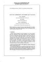
To graphically illustrate the general development of forecast errors per coun-
try I also calculate the absolute di¤erence between the average forecast (i.e. the
“consensus” of forecasters) and the actual interest rate at t + 3 months and
t + 12 months. Results are charted in Figure 2. As one might expect, the 3
month errors are generally smaller than the 12 month errors. Errors and their
variation are particularly large for countries that experienced …nancial and eco-
nomic crisis during this period, Argentina in particular dramatically stands out.
The 1998 …nancial market crisis a¤ects several countries in the sample partic-
ularly Asian and developing economies. The consequences of this shock vary
substantially, however, with peak errors varying from 0.5%-point for Japan to
20%-point for Indonesia. The 2001 recession is also visible for a minority of ad-
vanced economies. Overall, forecast errors vary substantially per country (also
see Table 2) and show di¤erent variations over time.
12
0
20
40
60
80

98 99 00 01 02 03 04 05
Argentina
0.0
0.4
0.8
1.2
1.6
98 99 00 01 02 03 04 05
Australia
0.0
0.5
1.0
1.5
2.0
98 99 00 01 02 03 04 05
Canada
0
1
2
3
98 99 00 01 02 03 04 05
Chile
0
2
4
6
8
98 99 00 01 02 03 04 05
Czech Republic
0.0

0.5
1.0
1.5
2.0
2.5
98 99 00 01 02 03 04 05
Germany
0
1
2
3
4
98 99 00 01 02 03 04 05
Hong Kong
0
1
2
3
4
98 99 00 01 02 03 04 05
Hungary
0
1
2
3
98 99 00 01 02 03 04 05
India
0
5
10

15
20
98 99 00 01 02 03 04 05
Indonesia
.0
.1
.2
.3
.4
.5
.6
98 99 00 01 02 03 04 05
Japan
0
2
4
6
8
98 99 00 01 02 03 04 05
Malaysia
0
1
2
3
4
98 99 00 01 02 03 04 05
Mexico
0
1
2

3
4
98 99 00 01 02 03 04 05
New Zealand
0
1
2
3
4
5
98 99 00 01 02 03 04 05
Norway
0
2
4
6
8
98 99 00 01 02 03 04 05
Poland
0
1
2
3
4
98 99 00 01 02 03 04 05
Singapore
0
2
4
6

8
98 99 00 01 02 03 04 05
Slovakia
0
2
4
6
8
98 99 00 01 02 03 04 05
South Korea
0.0
0.5
1.0
1.5
2.0
2.5
98 99 00 01 02 03 04 05
Sweden
0.0
0.4
0.8
1.2
1.6
2.0
2.4
98 99 00 01 02 03 04 05
Switzerland
0
2
4

6
8
10
12
98 99 00 01 02 03 04 05
Thailand
0.0
0.5
1.0
1.5
2.0
98 99 00 01 02 03 04 05
UK
0
1
2
3
98 99 00 01 02 03 04 05
t+3 t+12
USA
Figure 2: Absolute error of average forecast (%-point)
13
Figure 3 shows that patterns in the volatility data are analogous to those
described for the forecast errors. Here too the Asia crisis is visible, and again
there are substantial di¤erences in its impact. As with the errors data, di¤er-
ences between countries are large, both in terms of volatility levels (See Table
2) and variations over time.
The main di¤erence in Figure 3 versus Figure 2 is that the three month and
twelve month volatilities appear closer together than the corresponding errors
for these time frames. Given that the standard deviation of daily interest rates

is, by de…nition, calculated over a sample period, this is not surprising for two
reasons. First, the three month sample overlaps a quarter of the twelve month
sample. Second, the average date of the samples are closer together, i.e. t + 1:5
months and t + 6 months versus the t + 3 and t + 12 months for the forecast
errors.
14
0
4
8
12
16
20
24
28
98 99 00 01 02 03 04 05
Argentina
.0
.2
.4
.6
.8
98 99 00 01 02 03 04 05
Australia
.0
.2
.4
.6
.8
98 99 00 01 02 03 04 05
Canada

0.0
0.5
1.0
1.5
2.0
98 99 00 01 02 03 04 05
Chile
0
1
2
3
98 99 00 01 02 03 04 05
Czech Republic
.0
.2
.4
.6
.8
98 99 00 01 02 03 04 05
Germany
0.0
0.5
1.0
1.5
2.0
2.5
98 99 00 01 02 03 04 05
Hong Kong
0.0
0.5

1.0
1.5
2.0
98 99 00 01 02 03 04 05
Hungary
0.0
0.4
0.8
1.2
1.6
98 99 00 01 02 03 04 05
India
0
2
4
6
8
10
98 99 00 01 02 03 04 05
Indonesia
.00
.05
.10
.15
.20
.25
98 99 00 01 02 03 04 05
Japan
0.0
0.5

1.0
1.5
2.0
98 99 00 01 02 03 04 05
Malaysia
0
2
4
6
8
98 99 00 01 02 03 04 05
Mexico
0.0
0.2
0.4
0.6
0.8
1.0
98 99 00 01 02 03 04 05
New Zealand
0.0
0.5
1.0
1.5
2.0
2.5
98 99 00 01 02 03 04 05
Norway
0.0
0.5

1.0
1.5
2.0
2.5
98 99 00 01 02 03 04 05
Poland
0.0
0.4
0.8
1.2
1.6
98 99 00 01 02 03 04 05
Singapore
0
1
2
3
4
5
98 99 00 01 02 03 04 05
Slovakia
0.0
0.5
1.0
1.5
2.0
98 99 00 01 02 03 04 05
South Korea
.0
.1

.2
.3
.4
.5
.6
98 99 00 01 02 03 04 05
Sweden
.0
.2
.4
.6
.8
98 99 00 01 02 03 04 05
Switzerland
0
1
2
3
98 99 00 01 02 03 04 05
Thailand
0.0
0.2
0.4
0.6
0.8
1.0
98 99 00 01 02 03 04 05
UK
0.0
0.4

0.8
1.2
98 99 00 01 02 03 04 05
t+3 t+12
USA
Figure 3: Standard deviation of daily money market rates
15
Forecast errors and …nancial market volatility re‡ect more than just the
transparency of the central bank. Both are a¤ected by overall predictability of
interest rates due to the economic and …nancial risks that a¤ect them. To control
for country risk in the analysis below, I utilize the economic and …nancial risk
indicators of the International Country Risk Guide of the Political Risk Services
(PRS) Group. According to Linder and Santiso (2002) these ratings are used
by around four-…fths of the companies on Fortune magazine’s list of largest
multinationals. The …nancial and economics risk ratings are constructed with
objective data that are weighed together according to prede…ned scales.
5
Higher
ratings indicate less risk. The economic risk rating is constructed from GDP per
head, real GDP growth, in‡ation, general government balance as a percentage of
GDP and current account as a percentage of GDP. The components of …nancial
risk are foreign debt as a percentage of GDP, foreign debt service as a percentage
of exports of goods and services, current account as percentage of exports of
goods and services, o¢ cial reserves import cover and year-on-year exchange rate
movement. Es sentially the risk ratings provide a standardized and parsimonious
way to re‡ect a variety of economic and …nancial fundamentals that a¤ect risk.
A downside may be that the ratings may not re‡ect di¤erences in the ability
of countries to maintain government and current account de…cits or carry debt,
see for example the relatively low ratings of some developed countries in Figure
4 and Table 2.

5
See http:/ /www.prsgroup.com/PDFS/icrgmethodology.pdf.
16
15
20
25
30
35
40
45
98 99 00 01 02 03 04 05
Argentina
32
34
36
38
40
42
98 99 00 01 02 03 04 05
Australia
38
40
42
44
46
98 99 00 01 02 03 04 05
Canada
35
36
37

38
39
40
41
98 99 00 01 02 03 04 05
Chile
30
32
34
36
38
40
42
98 99 00 01 02 03 04 05
Czech Republic
38
39
40
41
42
43
98 99 00 01 02 03 04 05
Germany
36
38
40
42
44
46
48

98 99 00 01 02 03 04 05
Hong Kong
32
34
36
38
40
98 99 00 01 02 03 04 05
Hungary
28
32
36
40
44
48
98 99 00 01 02 03 04 05
India
15
20
25
30
35
40
98 99 00 01 02 03 04 05
Indonesia
35
40
45
50
98 99 00 01 02 03 04 05

Japan
28
32
36
40
44
98 99 00 01 02 03 04 05
Malaysia
3 5 .5
3 6 .0
3 6 .5
3 7 .0
3 7 .5
3 8 .0
3 8 .5
3 9 .0
98 99 00 01 02 03 04 05
Mexico
28
32
36
40
44
98 99 00 01 02 03 04 05
New Zealand
42
44
46
48
50

98 99 00 01 02 03 04 05
Norway
32
34
36
38
40
42
98 99 00 01 02 03 04 05
Poland
42
44
46
48
50
52
98 99 00 01 02 03 04 05
Singapore
28
30
32
34
36
38
40
98 99 00 01 02 03 04 05
Slovakia
28
32
36

40
44
48
98 99 00 01 02 03 04 05
South Korea
32
36
40
44
48
98 99 00 01 02 03 04 05
Sweden
40
42
44
46
48
50
98 99 00 01 02 03 04 05
Switzerland
24
28
32
36
40
44
98 99 00 01 02 03 04 05
Thailand
34
36

38
40
42
44
98 99 00 01 02 03 04 05
UK
28
32
36
40
44
98 99 00 01 02 03 04 05
Economic risk Financial risk
USA
Figure 4: Political Risk Services indices
17
Country Average Average Average Average Average Average
|Error| |Error| Volatility Volatility Risk Rating Risk Rating
t+3 t+12 t to t+3 t to t+12 Economic Financial
USA 0.4 1.2 0.2 0.5 40.1 35.2
Norway 0.7 1.4 0.3 1.0 46.7 47.1
Switzerland 0.4 1.2 0.2 0.3 44.3 46.1
Canada 0.5 1.1 0.2 0.4 42.5 40.3
Japan 0.1 0.2 0.1 0.1 37.9 46.8
Hong Kong 0.7 1.4 0.5 0.7 43.3 43.9
Australia 0.3 0.7 0.1 0.3 40.5 35.3
Germany 0.3 1.0 0.1 0.3 40.5 40.4
Sweden 0.4 0.8 0.1 0.3 43.7 37.5
UK 0.5 1.2 0.1 0.3 40.0 38.5
Singapore 0.9 1.0 0.4 0.5 47.3 45.4

N. Zealand 0.8 1.1 0.4 0.6 40.2 30.2
Korea, S. 1.3 1.6 0.3 0.4 40.6 38.9
Czech Rep. 0.6 2.3 0.1 0.6 34.4 39.3
Hungary 0.9 1.6 0.3 1.1 34.4 36.6
Slovakia 1.6 2.1 0.7 1.1 32.5 36.8
Argentina 18.3 32.7 3.6 8.4 34.5 26.3
Chile 1.0 1.2 0.4 0.5 38.9 37.3
Poland 2.1 3.3 0.5 1.2 34.7 38.8
Mexico 1.1 2.4 1.4 2.2 37.0 36.9
Malaysia 0.5 1.1 0.5 0.8 38.9 40.1
Thailand 2.0 2.8 0.9 1.3 38.0 38.6
Indonesia 2.2 4.5 0.5 1.8 31.8 31.1
India 0.7 0.9 0.4 0.6 33.6 40.9
Average 1.6 2.9 0.5 1.1 39.0 38.7
High 18.3 32.7 3.6 8.4 47.3 47.1
Low 0.1 0.2 0.1 0.1 31.8 26.3
Table 2: Absolute average error, volatility and risk ratings
18
4 A simple theoretical approach to public and
private information
Here I describe how transparency might have either a positive or negative e¤ect
on predictability in a very general but formal way. Along the lines of the dataset
employed below, consider a number of central banks, each with an accompanying
set of professional forecasters who make predictions of future policy rates.
A simple way to think about individual forecasts is as combinations of public
and private information, which are both noisy signals of future policy rates.
The noise in the signals are random errors that are assumed to be unbiased
and indep endently normally distributed. In the context of the data used, these
signals have a year index, t, but I suppress the subscript in this section b ecause
it applies to all variables.

(1) y
k
= b
k
+ !
k
!
k
= N

0;
1
p

k

Where
y public signal
b future policy rate
!
k
error of public signal for country k
k country index
 precision of public signal error (i.e. inverse of the variance)
(2) p
i;k
= b
k
+ !
i;k

!
i;k
= N

0;
1
p
s
i;k

Where
p
i;k
private signal of forecaster i for country k
i forecaster index
!
i;k
error of private signal of forecaster i for country k
s
i;k
precision of private signal error (i.e. inverse of the variance)
Assuming the forecaster aims to maximize accuracy, knows the precisions of
the public and private signals, and behaves rationally, the individual forecast,
f
i;k
, will be a combination of private and public signals, using relative precisions
as weights.
(3) f
i;k
=


k

k
+s
i;k
y +
s
i;k
+s
i;k
p
i;k
The error of the individual forecast with the future interest rate, 
i;k
, is
derived by subtracting b from the forecast.
19
(4) 
i;k
= f
i;k
 b
k
=

k

k
+s

i;k
!
k
+
s
i;k
+s
i;k
!
i;k
A convenient property of signals with normally and independently distrib-
uted errors is that the combined signal has a precision that is the sum of the
precisions of the individual signals. Equation (5) thus represents the precision
of the forecast error, 
i;k
.
(5) 
i;k
= 
k
+ s
i;k
It seems likely that transparency will increase the precision of the public
information. Equation (6) de…nes 
k
to be a function of transparency ( ) and
some other determinants D
k
.
(6) 

k
= 

(+; D
k
)
Where
 transparency
D
k
vector of other determinants of the precision of public information
It is less clear if transparency will a¤ect private information. In Equation
(4) the weight on public information will increase as it becomes more precise
and the weight on private information will decline, while the precision of private
information will remain unchanged. It may be the case, however, that the preci-
sion itself is also a¤ected. In line with the reasoning of Morris and Shin (2002),
agents may partially ignore their own private information because the public
signal acts as a coordinator of second degree expectations and thus becomes
over-emphasized in determining the resale value of the asset. Kool et al. (2011)
also raise the possibility that when private information is costly individual fore-
casters will invest less in the precision of the private signal. Both cases imply a
negative relationship between transparency and private information.
(7) s
i;k
= 
s
(; D
i;k
)
As a result, the relationship between transparency and predictability will be

a function of transparency’s separate e¤ects on the public and private signals.
(8) 
i;k
= 

(+; D
k
) + 
s
(; D
i;k
)
Kool et al. (2011) show that in a rational expectations asset market the
a¤ect of transparency on volatility is theoretically the same as its a¤ect on
predictability. They show that transparency can crowd out private information
and thereby both hurt predictability and push up volatility.
It is quite possible that in order to closely model the relationship between
transparency and the precisions of private and public information a more com-
plex setup would be required. For example, to represent the idea of Dale et al.
(2008) that forecasters may misestimate the precision of the public signal would
20
require adjusting the above equations to make a distinction between the actual
precisions and those that the forecasters perceive and thus use as weights. Fur-
thermore, Berger et al. (2006) note that forecasters di¤er in their analysis of
public information, indicating some complementaries between public and pri-
vate data. More generally, the approach used here requires assuming rational
agents that are able to optimally combine information, precluding the type of
confusion from multiple signals found in Ehrmann and Fratzscher (2007). These
papers indicate that the simple approach employed here leaves many paths unex-
plored. However, it is not my intention to construct a unifying theoretical model

that could incorporate all potential adverse e¤ects of greater transparency. In-
stead my goal is to provide a basic theoretical benchmark for interpreting the
econometric results presented in the next section.
5 Evidence
Below I present regression results for the relationship between transparency
and forecaster errors, followed by similar analysis for transparency’s impact
on interest rate volatility. First, however, I present two graphs to illustrate
the cross-country relationship of transparency with both forecast accuracy and
volatility. Both the graphs and the econometric evidence point to the conclusion
that transparency helps to improve accuracy and reduce volatility.
5.1 Cross section graphs
Graphs o¤er an intuitive way to illustrate the consequences of transparency for
predictability and interest rate volatility. Their downside is that any relationship
that is visually apparent may not stand the scrutiny of econometric analysis.
However, as I present such analysis in subsequent sections, it is a useful …rst step
to show that at least the super…cial relationships one would expect are present in
the cross-section of the data. Assuming that negative e¤ects of transparency on
private information do not dominate, countries with higher transparency should
have lower absolute forecast errors and lower interest rate volatility. Indeed, that
is what the scatter plots presented in Figures 5 and 6 suggest.
The graphs show a dot for each country in the sample except Argentina,
which has average errors and volatility well above that of the other countries
(See Table 2). Rather than looking at a speci…c year, the levels of transparency,
forecast errors and volatility are averaged over the …ve years of the sample.
I focus on the 3-month forecasts and volatilities. The black lines represent
ordinary least squares linear regressions …tted on the datapoints shown.
21
Figure 5: Transparency and forecast accuracy, country cross section
22
Figure 6: Transparency and interest rate volatility, country cross-section

5.2 Forecast accuracy
Having illustrated graphically that the cross-section shows a negative relation-
ship between transparency and both forecast errors and interest rate volatil-
ity, the next step is to utilize the full panel for a more complete econometric
analysis that controls adequately for country features other than central bank
transparency. This section does this for forecast errors and the next one for
interest rate volatility.
The results shown below are obtained from the following panel regression
for the individual forecast errors.
23