Approaches to Scaling of Trace Gas Fluxes in Ecosystems potx

vii
FOREWORD
The world's terrestrial and aquatic ecosystems are important sources of a number of
greenhouse gases and aerosols which cause atmospheric pollution and disturb the energy
balance of the Earth-atmosphere system. In recent decades the measurement techniques and
instrumentation for quantifying gas fluxes have been improved considerably. Yet, the
uncertainties in the regional and global budgets for a number of atmospheric compounds have
not been reduced due to the large spatial heterogeneity and temporal variability of the factors
that control gaseous fluxes in ecosystems.
Techniques used for extrapolating measurements or properties and constraining results
between different temporal and spatial scales are nowadays referred to as "scaling". All
scaling methods are embedded in the data. Apart from uncertainties associated with the data
used, errors may be caused by generalization of the basic data (e.g. in soil maps, ocean maps).
Moreover, much of the spatial and temporal variation at a detailed level is obscured as a result
of aggregation. Possible errors caused by the use of aggregated or generalized data in models
are generally not explicitly analyzed.
An important step in scaling of gas exchanges between ecosystems and the atmosphere is
the delineation of functional types where distinct differences in structure, composition or
properties of landscapes or water bodies coincide with functions or processes relevant for gas
fluxes. Delineation reduces the variability of state variables, and therefore functional types
form a good basis for measurement strategies and model development.
Models are widely used tools in bottom-up scaling approaches. Models can also be used to
calculate flux values for regions where less intensive or no measurement data are available.
One of the challenges in model development is the integration of properties or variables in
space and time, accounting for the spatial and temporal variability of processes involved in
gas production, consumption and exchange.
Scaling not only comprises bottom-up approaches, but also top-down methods, such as
inverse modelling to calculate from the atmospheric concentrations back to the sources. Top-
down scaling in general involves the validation of estimates obtained at a lower scale level
against constraints given at a higher level of scale. Hence, scaling requires uncertainty analysis

at all levels considered.
The present book is a collective effort of a diverse group of scientists to review the state-
of-the art in the field of scaling of fluxes of greenhouse gases and ozone and aerosol
precursors. It focuses on identification of gaps in knowledge, and on finding solutions and
determining future research directions. The book is the result of an international workshop on
"Scaling of trace gas fluxes between terrestrial and aquatic ecosystems and the atmosphere",
held from 18-22 January 1998 at kasteel "Hoekelum", Bennekom, the Netherlands. The
workshop was organized by the International Soil Reference and Information Centre (ISRIC)
as a follow-up to the international conference on "Soils and the Greenhouse Effect" which
ISRIC organized in 1989.
The overall goal of the workshop was to investigate approaches to reduce uncertainties in
estimates of fluxes of trace gases and aerosols between terrestrial and aquatic ecosystems and
the atmosphere at the landscape, regional and global scale. To achieve that goal, the
participants concentrated on: (i) Identification of data gaps in scaling approaches between
viii
field, landscape, regional and global scales; (ii) Development of procedures to bridge process
level information between different scales; (iii) Assessment of methods for integration,
aggregation and other data operations; and, (iv) Assessment of approaches to uncertainty
analysis in bottom-up and top-down scaling.
The workshop was one of researchers with many different backgrounds, including soil
science, microbiology, oceanography, rec.ote sensing and atmospheric sciences. The group
included experts in the determination of gas fluxes, modellers, specialists in the use of
isotopes and tracers, and researchers working on the compilation of regional and global
inventories and maps of soils, vegetation, land use and emissions.
Twelve invited background papers, providing a review of the field, were distributed prior to
the workshop, but were not presented at the meeting. Instead, the scientific programme of the
workshop consisted of five days of discussions according to the well-known Dahlem
workshop model. The participants were divided in four interdisciplinary working groups
which met to address the workshop aims and give concise and practical recommendations,
concentrating on the following questions: (i) How can fluxes of trace gas species be validated

between different scales ?; (ii) How can we best define functional types and integrate state
variables and properties in time and space ?; (iii) What is the relation between scale, the
model approach and the model parameters selected ?; (iv) How should the uncertainties in the
results of scaling be investigated ? The four group reports are included in this volume as
separate chapters together with the peer-reviewed background papers.
The organizing committee for the workshop, which started discussions Jn 1996, included
the following members: A.F. Bouwman (National Institute of Public Health and the
Environment, Bilthoven), N.H. Batjes (International Soil Reference and Information Centre,
Wageningen), H.A.C. Denier van der Gon (Soil Science and Geology Department, Wageningen
Agricultural University), F.J. Dentener (Institute for Marine and Atmospheric Research,
Utrecht University), J. Duyzer (TNO Institute of Environmental Sciences, Energy Research and
Process Innovation, Apeldoorn), W. Helder (Netherlands Institute for Sea Research, Den Burg),
J. Middelburg (Netherlands Institute of Ecology, Centre for Estuarine and Coastal Ecology,
Yerseke).
The organization of the workshop was made possible through funds of the Commission of
the European Communities (CEC-DG XII), European IGAC Office (EIPO), International
Fertilizer Industry Association (IFA), Kemira Agro Oy, National Institute of Public Health
and the Environment (RIVM), Norsk Hydro, Netherlands Royal Academy of Arts and
Sciences (KNAW), Shell Nederland b.v., and the Netherlands Organization for Applied
Scientific Research (TNO).
Cooperating organizations were the Intemational Society of Soil Science (ISSS),
International Geosphere-Biosphere Programme (IGBP), International Global Atmospheric
Chemistry Programme (IGAC), Global Emission Inventories Activity (GEIA), Centre for
Climate Research (CKO), and the Climate Change and Biosphere Programme of the
Wageningen Agricultural University (CCB)
Dr. L.R. Oldeman
Director, Intemational Soil Reference and Information Centre (ISRIC)
October 1998
ix
ACKNOWLEDGEMENTS

This volume is the result of an international workshop on "Scaling of trace gas fluxes between
terrestrial and aquatic ecosystems and the atmosphere", held from 18-22 January 1998 at
kasteel "Hoekelum", Bennekom, the Netherlands. It is a collective effort of a diverse group of
scientists. The choice of topics, identification of authors for the invited background papers,
and the scientific programme around four key questions is the result of discussions in the
organizing committee. Thanks are due to the members of this committee, Niels Batjes, Hugo
Denier van der Gon, Frank Dentener, Jan Duyzer, Wim Helder and Jack Middelburg. Thanks to
the enthusiastic involvement of the committee members the workshop became a very success-
ful one.
I wish to thank the chairmen and rapporteurs of the four working groups for leading the
discussions and summarizing the various contributions of the working group members in four
reports which are included in this book: Andi Andreae and Willem Asman (group I), Jean-
Paul Malingreau and Sybil Seitzinger (group 2), Peter Liss and Jack Middelburg (group 3),
Arvin Mosier and Dick Derwent (group 4).
I am indebted to all participants for reviewing the invited background papers. Carl
Brenninkmeier, who could not attend the meeting, was so kind to provide a review of one of
the papers. I am also thankful to Niels Batjes for critically reading two papers, and to Ruth de
Wijs-Christensen of RIVM for editing one of the background papers.
I very much appreciated the support and ideas of Roel Oldeman Hans van Baren of ISRIC
during the preparation of the workshop. Special thanks are due to Jan Brussen, Yolanda
Karpes-Liem and Hans Berendsen for their enthusiasm and input during the preparations of
the workshop and the workshop. Finally, I am grateful to Wouter Bomer for designing the
workshop logo (also presented on the cover of this book) and for preparing some of the
figures in the book.
Finally, I wish to thank Fred Langeweg of RIVM for giving me the opportunity to work on
this projectl
Lex Bouwman, editor
October 1998
Approaches to scaling a trace gas fluxes in ecosystems
A.F. Bouwman, editor

9 Elsevier Science B.V. All rights reserved
TOWARDS RELIABLE GLOBAL BOTTOM-UP ESTIMATES OF TEMPORAL
AND SPATIAL PATTERNS OF EMISSIONS OF TRACE GASES AND AEROSOLS
FROM
LAND-USE RELATED AND NATURAL SOURCES
A.F. Bouwman l, R.G. Derwent 2 and F.J. Dentener 3
~ National Institute of Public Health and the Environment, P.O. Box 1, 3720 BA Bilthoven, The Netherlands
2 Meteorological Office, London Road, Bracknell, RG 12 2SZ Berkshire, UK
3 University of Utrecht, Institute for Marine and Atmospheric Research, Princetonplein 5, 3584 CC Utrecht, The
Netherlands
I. Introduction
Emission inventories play a dual role in global air pollution issues. Firstly, they can be used
directly to establish the more important source categories, to identify trends in emissions and
to examine the impact of different policy approaches. Secondly, emission inventories are used
to drive atmospheric models applied to assess the environmental consequences of changing
trace gas emissions and concentrations and to provide advice to policy makers. This second
role contributes to the atmospheric modelling community being an important user of emission
inventories. The assessment process for global air pollution problems has a number of
identifiable steps: (i) it quantifies the changes in trace gas composition of the atmosphere; (ii)
it quantifies changes in atmospheric chemistry, transport, deposition and radiative forcing;
(iii) it identifies the climate responses to the changes in atmospheric composition of the
radiatively active trace gases; and, (iv) it quantifies the biological and ecological responses to
the predicted changes in climate.
The atmospheric modelling community will need a hierarchy of emission inventories to
complete an assessment of global air pollution problems based on these steps over the next
decade or so. In their simplest form, atmospheric models merely require no more than fixed
global emission fields of each relevant species. However, in their most complex form, future
atmospheric models will require emission fields whose spatial patterns and magnitudes will
respond in a wholly self-consistent manner to changes in economic prosperity, demography,
land use, climate change and policy. The requirements placed on the emission inventories will

change from the provision of fixed fields to the implementation of emission algorithms within
the modelling system. Gridded emission fields may slowly change from being the essential
input to being the output of the modelling system.
Alongside this anticipated increase in complexity in moving towards a process-based
approach to emission inventories, there is a growing interest in the emissions of a wider range
of species. For example, in climate change research at the start of the Intergovernmental Panel
on Climate Change (IPCC) process, assessment work was performed with present-day and
doubled atmospheric carbon dioxide (CO2) concentrations. This "steady state" or
"equilibrium" approach has now been replaced by the transient scenario approach in which
CO2 concentrations increase with time in response to emission projections and carbon cycle
modelling. Further scenarios have been added to deal with the other major radiatively active
trace gases: methane
(CH4),
nitrous oxide (N20), tropospheric ozone (03), stratospheric ozone
4
A.F. Bouwman, R.G. Derwent and F.J. Dentener
Table 1. Some recent global-scale chemistry-transport r .tels (types, spatial and time scales and che :'ical mechanisms),
Model Type Spatial resolution of Time resolution of Chemical Re-
meteorological data meteorological data mechanism ference a
GETTM Eulerian 2.8~215176215 18 levels 3-hourly radioactive decay 1
GEOS-I DAS Eulerian 2.5%2~215 levels 6-hourly Simplified 2
GFDL/GCTM Eulerian 265 km• kmxl I levels 6-hourly Simplified 3
GISS/CTM Eulerian 4~215 levels 4-hourly to 5-day DMS chemistry 4
GRANTOUR Lagrangian 7.5~215 12 levels 12-hourly 76 species 5
IMAGES Eulerian 5%5~215 levels monthly 47 species 6
IMARU Eulerian 3.75%3.75% 19 levels 1/2-hourly CH4 and NO• 7
chemistry
KFA/GISS Eulerian 10%8% 15 levels 8-hourly Simplified 8
KNMI/CTMK Eulerian 2.5%2.5~ 15 levels 12-hourly 13 species 9
MCT/UiB Eulerian 150 kmx 150 kmx 10 levels hourly 51 species 10

MOGUNTIA Eulerian 10~ 10% 10 levels monthly CH4 and NOx 11
chemistry
MOZART Eulerian 2.8%2.8% 18 levels 6-hourly 45 species 12
RGLK Eulerian 10~ 10% 0 levels Monthly SO2, NOx and NH3 13
chemistry
STOCHEM Lagrangian 3.75~215 19 '. ~els 6-hourly 70 seecies 14
UiO/GISS Eulerian 8~ 10~ levels 8-hourly to 5-day 50 species 15
a 1, Li and Chang (1996); 2, Allen
et al.
(1996); 3, Moxim
et al.
(1996); 4, Chin
et al.
(1996); 5, Penner
et al.
(1994); 6,
Mt~ller and Brasseur (1995); 7, Roelofs and Lelieveld (1995); 8, Kraus
et al.
(1996); 9, Wauben
et al.
(1997); 10, Flatoy and
Hov (1996); 11, Dentener and Crutzen (1993); 12, Brasseur
et al.
(1997); 13, Rodhe
et al.
(1995); 14, Collins
et al.
(1997);
15, Berntsen
et al.

(1996).
and chlorofluorocarbons (CFCs). More recently, sulphur dioxide (SO2), dimethylsulphide
(DMS), ammonia (NH3) and other aerosol species have been incorporated into the scenario
approach to take into account the climate consequences of man-made fuel combustion and
biomass burning. There has therefore been an increasing interest in the details of the emission
inventories of a wider range of trace gases and aerosols.
Emission inventories are implemented in current atmospheric models to represent the
processes by which trace gases and aerosols are discharged into the model atmosphere. The
models, commonly three-dimensional chemistry transport models (CTMs), then simulate the
dispersion, diffusion and advection of thi material away from its source r~'gions in response
to a continuously varying turbulent and chaotic atmospheric flow. At some point, the material
may be removed from the atmospheric circulation by dry or wet deposition or uptake in the
oceans or it may undergo chemical transformation. An immense amount of meteorological,
chemical and process information is required to drive current CTMs. This information can be
made available from archived meteorological analyses or from the global climate models
(GCM) used to predict future climate change. The CTM may be incorporated within the
GCM, in which case the atmospheric model is "on-line"; alternatively, the model is referred to
as "off-line" if the GCM and CTM are separated. By way of example, details of the time and
spatial resolution of 15 of the current CTMs are provided in Table 1. At present some 20
CTMs are being used to assess global air pollution problems. Currently, CTMs use emission
inventories for the trace gases and aerosol species listed in Table 2. Each emission is usually
subdivided into up to about 10 major source categories. Most source categories have different
spatial grids applied and work with different seasonal and sometimes diurnal variations.
We will focus here on the issues of "scaling" in the implementation of emission inventories
in current and future CTMs. Scaling comprises all techniques used for extrapolating
measurements or properties and constraining results between different temporal and spatial
scales. Very similar problems of scaling occur across various disciplines, such as ecology
(Ehleringer and Field, 1993), soil science (Wagenet and Hutson, 1995; Hoosbeek and Bryant,
Towards reliable global estimates of emissions of trace gases and aerosols 5
Table

2. Some of the trace gases and aerosol species handled by current chemistry transport models (CTMs) for the
assessment of global air pollution problems.
Radiatively active gases Aerosols
CO2 Black carbon
CH4 Organic particles
N20 Wind-blown dust
CFCs: 11,12,113 Sea-salt
HCFCs: 22, 141b, 142b Resuspended material
HFCs: 134a, 152a Volcanic emissions
Perfluoro molecules: SF6, CF4, C2F6, C4F8 Biomass burning
Ozone precursor and depleting gases Aerosol precursor gases
CO SO2
NOx DMS
H2 H2S
Synthetic hydrocarbons: light C2 - C~o hydrocarbons, NH3
oxygenates
Biogenic hydrocarbons: isoprene, terpenes
CH3CC13, C2C14, C2HC13, CH2C12
CH3Br
CH3CI
Synthetic bromine compounds: 12B 1, 13B 1
1992) and global change research in general (O'Neill, 1988).
Two approaches are used for scaling gas fluxes: bottom-up and top-down scaling. Bottom-
up approaches, calculated from smaller to larger scales, involve extending calculations from
an easily measured and reasonably well understood unit to more encompassing processes. In
bottom-up scaling, various problems occur, such as how to aggregate the spatial and temporal
variation of properties or fluxes. Other problems are the various data uncertainties involved,
and translating mechanisms and processes between different scales.
Top-down approaches can mean using the measurements at a higher scale level which set
the boundary conditions for problem identification, and stimulate the testing of general

relationships for specific cases (see Heimann and Kaminski, 1999). Examples of observations
at a higher level of scale that are used to constrain flux estimates include atmospheric
concentrations and mixing-ratios of stable isotopes (see Trumbore, 1999). Comparison of the
concentrations or deposition velocities simulated by transport models with observations can
result in an expression of scientific confidence or a warning that crucial !r, formation is still
missing. Between these two extremes, top-down scaling can be very useful for testing
hypotheses and identifying missing information.
A number of methods exist to scale information, the most important being aggregation,
generalization, stratification and modelling. Aggregation involves the collection or uniting of
information into an aggregate unit, generally by counting and addition. Aggregated results can
be presented as the mean or median coupled with statistical information such as standard
deviations.
Generalization is the description of a group on the basis of properties of a sub-unit or
member of the group considered to be representative, commonly based on expert knowledge.
This method is generally used when observational or statistical data on individual members of
the group are scarce.
The reverse action of aggregation, whereby the aggregate is subdivided into different
components, may be the classification of a system into functional units with similar properties
and environmental and management conditions that regulate trace gas fluxes (see Seitzinger
et
al.
(1999). This is sometimes referred to as "stratification" (Matson
et al.
(1989).
6
A.F. Bouwman, R.G. Derwent and F.J. Dentener
Models break down a system into its main components and describe the behaviour of the
system through the interaction of those components. A discussion of the different types of
models used can be found in Archer (1999) for aquatic systems and Schimel and Panikov
(1999) for terrestrial systems.

We will focus here on bottom-up scaling approaches for trace gas fluxes between aquatic
and terrestrial ecosystems (including agroecosystems) and the atmosphere used in the develo-
pment of global gridded emission inventories. The discussion will be primarily on emission
inventories prepared for scientific purposes such as atmospheric modelling. Although our
findings may also hold for other types of inventories, we will not discuss these inventories
explicitly on the country or provincial (sub-national) scale. Such inventories are now being
prepared for non-scientific purposes (e.g. national communications in the United Nations
Framework Convention on Climate Change).
The first, and major, part of this paper discusses the uncertainties and problems of
aggregation, generalization, stratification and modelling in the compilation of inventories.
Next, the available global emission inventories for land-use related and natural sources of
trace gases will be discussed on the basis of their spatial and temporal resolution. Finally, the
spatial and temporal resolution of current CTMs will be confronted with the available
emission inventories.
2. Uncertainties in emission estimates
Among the various approaches to estimating fluxes, the major ones in use are the emission
factor approach and modelling. In emission factor approaches emission estimates are derived
by combining measurement data with geographic and statistical information on the ecosystem
processes and economic activity. This can be represented as:
E= A • Eu
(1)
where E is the emission, A the activity level (e.g. area of a functional unit, animal population,
fertilizer use, burning of biomass) and
EU
the emission factor (e.g. the emission per unit of
area, animal, unit of fertilizer applied or biomass burnt). When using the emission factor
approach, both the stratification scheme for delineating functional types (e.g. management
systems, ecosystems, environmental provinces or entities) as a basis fol scaling, and the
reliability of the emission factor determine the accuracy of the flux estimates.
The firmest basis for scaling is developing an understanding of the mechanisms that

regulate spatial and temporal patterns of processes, and describing these mechanisms in
models. Models are used to break down a system into its component parts and describe the
behaviour of the system through their interaction. In general, trace gas flux models include
descriptions of the processes responsible for the cycling of carbon or nitrogen and the fluxes
associated with these processes. Various types of models exist, including regression models,
empirical and process (or mechanistic) models.
In the following sections the various sources of uncertainty in the estimates of emission
rates for the emission factor approach, trace gas flux models and farm-scale models will be
discussed, followed by uncertainties associated with the spatial and temporal distribution of
the data underlying flux estimates. We will not discuss uncertainties in the measurement data.
This problem will be examined in more detail by Lapitan
et al.
(1999), Fowler (1999),
Denmead
et al.
(1999) and Sofiev (1999).
Towards reliable global estimates of emissions of trace gases and aerosols 7
2.1. Uncertainties in the emission rates
2.1.1. Emission factor approach
Uncertainty ranges for emission inventories are usually presented for the global total emission
only, and not on a regional or grid-by-grid basis. Uncertainties in emission inventories may be
caused by uncertainties in the environmental and economic activity data used and in the
measurement data themselves. Uncertainties can also result from the lack of representative
measurem'ents to resolve the full range of ,mvironmental conditions occurrhag in the systems
considered and in the models used. These sources of uncertainty will be discussed for the
different approaches to flux estimation on the basis of a number of examples for different
scales.
- Measurement data.
In a review of measurement data for biomass burning, Andreae
(1991) proposed emission factors for several gas species. Although the ranges in measured

fluxes in field and laboratory experiments varied by more than a factor of 2 for most species
as a result of differences in fuel and burning conditions, one single emission factor was
proposed for each gas species, representing the aggregated flux for smouldering and flaming
fires for all fuel types (grass, wood, crop residues, etc.). For biomass burning it is difficult to
delineate the types of fires and the different techniques used may introduce systematic
differences, especially where reactive and difficult-to-measure species (such as NOx and NH3)
are involved. Clearly, one emission factor cannot describe all the burning conditions and fuel
types.
Another example illustrating the lack of measurement data concerns the emission
coefficients used for animal housings in Europe. In housings with mechan!cal ventilation the
gas flux can be easily determined from the gas concentration in the ventilation air and the flow
rate. The trace gas emissions from naturally ventilated housings can only be determined
indirectly and with greater uncertainty. In such "open" housings the emission depends on the
opening and closing of doors. In large parts of Europe, housings for cattle - the most important
category- are naturally ventilated (Asman, 1992). Besides being scant, the available
measurement data need not be representative. For example, the NH3 ammonia emission per
animal may vary by a factor of 4 within the same type of housing (Pedersen
et al.,
1996). This
may be caused by differences in the ventilation over the slurry between housings and by
differences in waste management practices such as cleaning.
Guenther
et al.
(1995) were also confronted by a lack of measurement data in their global
invemory of fluxes of volatile organic compounds (VOC) from vegetation. Measurements
represented only 26 of the 59 global land-cover types considered; the remaining land-cover
types, including tropical seasonal forests and savannas, were assigned an emission on the
basis of expert knowledge. In this database, most of the simulated VOC emissions come from
systems where very few or no measurements are available.
- Functional types. Guenther

et al.
(1994) proposed emission factors for VOC for 91
woodland landscapes in the USA by combining emissions from 49 genera of plants. In their
global modelling ofVOC, Guenther
et al.
(1995) used emission factors on the basis of the 59
land-cover types defined by Olson
et al.
(1985). This aggregation causes considerable loss of
information, as the detailed estimates for the USA vary by as much as a factor of 5 for various
aggregated landscapes on the global scale.
Yienger and Levy II (1995) used a combination of emission factors and modelling
approaches to estimate global emissions of NO from soils. They first calculated "biome
factors" based on NO flux estimates from the literature. These biome-dependent average
fluxes were modified by an algorithm to account for pulse events of NO production following
8 A.F. Bouwman, R.G. Derwent and F.J. Dentener
wetting of dry soil and another algorithm to account for the effect of varying temperature.
Yienger and Levy (1995) also made an attempt to model the effects of NOx uptake by plants
on net NOx emission to the atmosphere. They calculated absorption factors based on leaf area
indices, and then multiplied these absorption factors by the estimated soil emissions to
calculate net ecosystem emissions. The model of Yienger and Levy has some mechanistic
components, such as the wetting and temperature functions, but is primarily based on
averaged biome factors that are not substantially different from an emission factor approach.
Davidson and Kingerlee (1997) also derived emission factors based on data for biomes
from the literature. Although in their study more soil NOx measurement data were used in
comparison to Yienger and Levy's study (1995), the major differences between the two
studies are the stratification scheme and t;L,~ coupling of environmental con.~ition descriptions
at the measurement sites with the functional types distinguished. Davidson and Kingerlee
(1997) presented a global annual emission which exceeds the estimate of Yienger and Levy
(1995) by a factor of 2. It is clear that the differences between the two studies described will

have an enormous impact on the results of atmospheric models.
2.1.2. Regression approaches
Bouwman
et al.
(1993) calculated the N20 emission from soils under natural vegetation using
a simple global model describing the spatial and temporal variability of the major controlling
factors of N20 production in soils. The basis for the model is the strong relationship between
N20 fluxes and the amount of nitrogen (N) being cycled through the soil-plant-microbial
biomass system. The model calculates the monthly N20 production potential from five indices
representing major regulators of N20 production (soil fertility, organic matter input, soil
moisture status, temperature and soil oxygen status). These five indices were combined in the
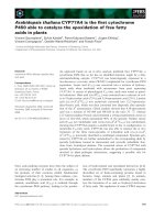
final N20 index (Figure 1). Comparison of the N20 index with reported measurements for
about 30 locations in six ecosystems correlated with an r 2 of- 0.6 (Figure l a). The resulting
regression equation was used to calculate emissions on a l~ 1 ~ resolution. However, the
correlation coefficient is not a robust statistical method (see Sofiev, 1999), and minor
differences in only one of the measurement sites can cause major shifts in the correlation
coefficient (Bouwman
et al.,
1993). A major problem causing unreliability of the regression
equation is the lack of measurement data, particularly for a number of important ecosystems
and world regions that have not been sampled at all. It is not known how the model performs
in these areas (Figure 1 b).
2.1.3. Process models
Reliable regional or global estimates of trace gas emissions depend on an examination of
methodologies to reduce the current high uncertainty in the estimates. One potential way to
do this is to develop predictive flux models. Such models have been developed for different
processes and gas species on different scales. Examples will be given of the magnitude of the
uncertainties in global models, the value 9f models developed for speci~c ecosystems for
extrapolation and the problem of selecting the appropriate scale of process descriptions in
models. Finally, the advantages of using a range of models on different scales will be

discussed.
-
Uncertainties in global flux models. Here, examples for oceanic flux models will be
given, although very similar examples also exist for terrestrial models. In aquatic systems,
fluxes can generally not be directly determined. Models commonly used describe fluxes on the
basis of wind speed and anomalies of concentrations between surface water and air. Nevison
et al.
(1995) calculated the air-sea exchange using three different relationships for the NzO-air
Towards reliable global estimates of emissions of trace gases and aerosols 9
550
450
-r 350
r
0
E
z 25O
6
z
~ 150
50
-50
a. Relation between measured NzO fluxes and modelled N20 index
o Measured flux
Regression equation
0
0 s 0
o
o o
o o
o oi" oO

o
i + ;
N20 index
b. Location of measurement
sites
90 90
-30 -
""" .,~. " - tc-' ~S'.: ~ .~
I"~ 1- : : ~, (~: .'%: " . "
~,.~-,,:,~: , :-~ ~ ~ ,: . ~ ,~) , ,,': . ~.~ ~,~ , -,,
" ;~ ' ~-~,~,,, - , ~=' "
.: ,~ , !
-:.:- ,~ .
9 . , :'~.',]:- , ' " ~: (., : _. -, ,,
:':
"~ : "-~ ~ " ~ "
-30
:: 6 .,.:
-60 - O
Measurement sites -
-60
, ,::':G- -
9 -
-90
-90
- -1 ,o 6 6'o
Figure 1. a) Relationship between measured N20 flux and simulated N20 index; and b) the location of the
measurement sites. Figure 1 a was modified from Bouwman et al. (1993) with kind permission from the American
Geophysical Union.
gas transfer velocity from global

N20
surface anomalies. The highest N20 fluxes were
obtained using a quadratic function of wind speed for the transfer velocity, while linear
functions yielded much lower values. An intermediate relationship was the stability-dependent
method based on the occurrence of whitecaps, also used by Guenther
et al.
(1995) for
estimating the VOC emission inventory for oceans. The uncertainty in the global emission is
illustrated by the difference of more than a factor of 4 between the lowest and the highest
global emission estimate.
-
Limitations of
ecosystem models.
Although models developed for specific ecosystems
may show fewer uncertainties than global models, their value for extrapolation may be
10
A.F. Bouwman, R.G. Derwent and F.J. Dentener
limited. Mosier and Parton (1985) developed a model for the estimation of N20 fluxes over
large areas of semi-arid grassland soils, accounting for spatial and interannual variability.
Model parameters were developed by relating N20 flux to soil moisture and temperature for
two sites representing much of the variability in the Colorado shortgrass ecosystem. Because
no time-series data of NO3 and NH4 + are available on the target scale of the study, the model
was simplified with an empirical multiplier representing N availability. It is especially
empirical multipliers like these that cause problems when models are applied to other
ecosystems with different environmental and climatic conditions.
-
Scale of process descriptions. Some models seem to include an imbalance in the detail
and the particular scale on which different processes are described. For example, Li
et al.
(1992) developed a model to simulate N20 fluxes from decomposition and denitrification in

soils on the field scale. The model can also describe NO• fluxes by using soil, climate and
data on management to drive three submodels (i.e. thermal-hydraulic, denitrification and
decomposition submodels). The management practices considered include tillage timing and
intensity, fertilizer and manure application, irrigation (amount and timing), and crop type and
rotation.
One of the processes simulated by the model is microbial growth. Since model results
appear to be dominated by the effect of temperature and soil moisture, which operate at nearly
all levels in the model, the question arising is whether there is an imbalance in the scales
according to which processes are described. The similarity of the results obtained for
shortgrass ecosystems by Mosier and Parton (1985) with their simple approach to those of Li
Simulated (g m "2)
75-
(a)
60-
45-
30-
15-
0 /
45
model correspondence
(rA2=0.905, n=36)
~
~o (:)
o
o o
O O
1"1 correspondence
(b)
model correspondence u~
(rA2=0.893, n=36)

oj 1"1 correspondence
~176
9 9 e
0 15 30 45 60 75
Measured (g m 2)
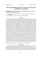
Figure 2. Comparison of simulated and measured total seasonal methane emissions from Texas flooded rice
paddy soils during the 1991-95 growing seasons employing consecutively (a) the simulation model and (b) the
simplified model. Model correspondence is the regression line of simulated vs. measured methane emissions.
Reprinted from Huang
et al.
(1998) with kind permission of Blackwell Science Ltd.
Towards reliable global estimates of emissions of trace gases and aerosols
11
et al.
(1992) illustrates the need to match the scale of process description with that of the scale
at which the model is applied. Comparisons of different models to predict N20 fluxes from
fields (Frolking
et al.,
1997) reveal major differences in the simulated N gas fluxes from soils.
Apparently, the major problem in developing trace gas flux models is the description of soil
processes that operate in "hot spots" in field models.
- Models at different scales.
Apart from the above-mentioned problem of the scale on
which processes operate, a very practical problem is formed by the available model input data.
To overcome this problem, sometimes summary models are developed on the basis of the
detailed process model. These summary models can be used to predict fluxes in regions with
limited data availability. Progress with the use of models on different scales for flooded rice
paddy fields was made by Huang
et al.
(1998). Understanding the processes of methane

production, oxidation and emission in flooded rice fields enabled them to develop a semi-
empirical model. They also derived a simplified (summary) version of the model for
application to a wider range of conditions but with limited data sets. Huang
et al.
(1998)
hypothesized methanogenic substrates as being primarily derived from rice plants and added
organic matter. Rates of methane production in flooded rice soils are determined by the
availability of methanogenic substrates a,~d the influence of environmemal factors. Model
validation against observations from single-rice growing seasons in Texas (USA)
demonstrated that the seasonal variation of methane emission is regulated by rice growth and
development. A further validation of the model against measurements from irrigated rice
paddy soils in various regions of the world, including Italy, China, Indonesia, Philippines and
the United States, suggested that methane emission could be predicted from rice net
productivity, cultivar character, soil texture and temperature, and organic matter amendments.
The detailed model and the summary model gave similar results (Figure 2), illustrating the
advantage of using simplified models.
2.1.4. Farm nutrient balance models
On the farm scale, trace gas fluxes occur in the stable, during grazing or during and after
spreading of animal manure. A model is therefore required to describe farm-scale processes
and cycles. For example, the model of Hutchings
et al.
(1996) describes NH3 losses from
animal housings, stored slurry, application of slurry and urine patches. The model builds on
knowledge acquired from various experiments and model studies of animal housing, waste
storage and farming practices. The model tracks the N input as animal feed until it is lost as
NH3. The problem of applying farm-scale models is the variety in management styles
occurring within groups of farms. Representative farms or averages for a group of farms have
to be used to obtain aggregated data. Differences in fluxes as a result of differences in
management may disappear due to this aggregation.
2.2. Uncertainties in the spatial distributions

The environmental spatial data used as a basis for stratification schemes for delineation of
functional types underpins the emission factor approach and, if sufficient attribute data are
available, drives flux models. When no spatial data are available to distribute activities or
emissions, a proxy or surrogate distribution has to be used. Clearly, this introduces an
unknown uncertainty in the spatial distribution. We will give a number of examples of
databases that describe environmental conditions in aquatic and terrestrial ecosystems,
emphasizing their uncertainties. A comprehensive review of the data required for global
terrestrial modelling can be found in Cramer and Fischer (1996). The list of examples given
12
A.F. Bouwman, R.G. Derwent and F.J. Dentener
here is not intended to be complete, but does illustrate data limitations and aggregation
problems. The weaknesses and strong points in the databases discussed may serve to improve
future database development. The examples considered include databases for climate, oceans,
soils and vegetation/land cover, as well as the problem of surrogate spatial distributions.
2.2.1. Climate
The example of a database on current climate for a global terrestrial 0.5 ~ x 0.50 grid given by
Leemans and Cramer (1991; update in preparation) includes average monthly, average
minimum and maximum air temperature, precipitation and cloudiness values.
-
Data limitations. The weather records were usually limited to at least five observational
years from the period of 1931-1960. Not all stations considered have complete coverage.
Based on selection criteria, the final number of stations worldwide was found to be 6280 for
temperature and 6090 for precipitation. The cloudiness data set, defined as the number of
recorded bright sunshine hours as a percentage of potential number, was based on fewer
stations and often derived from estimated rather than recorded data.
-
Aggregation. To aggregate the point data to a spatial grid an interpolation onto 0.5 ~ grid
boxes was done using a triangulation network followed by smooth surface fitting. For regions
with no primary data, the temperature val.aes were corrected for altitude using an estimated
moist adiabatic lapse rate and a global topography data set, while precipitation was not

corrected; this was due to the more complex relationships between precipitation and altitude.
- Uncertainty. The major problem is the inappropriate data coverage for large areas of the
world. The uncertainty of temperatures is particularly high in mountainous areas because there
are only a few weather stations in these regions and none of them are located on a clear
altitudinal gradient. The average moist adiabatical lapse rate for mountainous areas may result
in underestimation of temperatures for these areas. The spatial precipitation patterns resulting
from straight interpolation of measured values causes great uncertainty in areas with sparse
data coverage. Although the major annual cloud dynamics are represented, the regional
reliability of the cloudiness data is low.
2.2.2. Oceans
The best known chemo-physical global ocean data sets are included in the World Ocean Atlas
(Conkright
et al.,
1994; Levitus and Boyer, 1994a, b; Levitus
et al.,
1994). This database
includes spatial information on a l~ 1 ~ grid at various depths between 0 and 5500 m below
the surface for ocean temperature, salinity, dissolved oxygen, apparent oxygen utilization,
oxygen saturation, phosphate, and nitrate and silicate. Data for temperature and salinity have a
monthly time resolution and apply to depths between 0 and 1000 m below the surface; those
for dissolved oxygen, apparent oxygen utilization and oxygen saturation are on a seasonal
temporal scale and phosphate; nitrate and silicate concentrations taken on an annual basis.
-
Data limitations. The World Ocean Atlas is based on many observations. For example,
the temperature data set is based on 4.5 million profiles. Although the number of observations
is much higher than that used to produce the soil, vegetation/land cover and climate databases,
there is a problem of areas with a low density or absence of observations; furthermore, the
timing of the measurements may differ between profiles.
- Aggregation. The data at the observed depth were interpolated to standard depths. The
accuracy of the observed and standard level data was checked and flagged using a number of

procedures. The point data for depth profiles were interpolated onto a 1 o grid.
- Uncertainty.
There are many regions where measurements are scant or even absent. To
describe the density of observations, there are accompanying mask files for all the data listed
Towards reliable global estimates of emissions of trace gases and aerosols 13
above, containing the number of grid points with data within the radius of influence
surrounding each grid box. If a grid box contains three or fewer observations within its radius
of influence, the mask value for that 1 ~ grid box will be zero. This file is used in plotting
routines to "mask" or cover up areas with three or fewer observations.
2.2.3. Soils
Soil fertility, and soil chemical and physical parameters, play an important role in the
production and exchange of trace gases. Recently, a 0.5 ~ • 0.5 ~ global soil database was
developed on the basis of an edited version of the 1:5 million scale FAO Soil Map of the
World (FAO, 1991), combining geographic information on soil types with a set of
representative soil profiles held in a profile-attribute database (Batjes and Bridges, 1994).
-
Data limitations. The density of available soil profile data varies from one region to the
other. Important geographic gaps are in China, the New Independent States and the Northwest
Territories of Canada. Similarly, a number of soil units are underrepresented in the profile
database; these units account for about 28% of the terrestrial globe of which total Lithosols
(shallow soils) account for about 40%.
- Aggregation. The FAO Soil Map of the World is a compilation of many national and
regional soil maps. Therefore coverage is not spatially constant. The soil profile information
for each soil unit was coupled to the soil units distinguished region-wise. Based on the
number of profiles available, statistical analysis was performed by Batjes (1997), allowing
refinement of ratings for soil quality in global environmental studies.
-
Uncertainty. The variability of the reliability of the spatial information has already been
mentioned. The attribute files containing soil profile data in Batjes and Bridges (1994)
represent a major improvement on the FAO soil map as such. However, this aggregation may

not realistically describe the variability actually occurring within a soil unit in regions where
the density of observations is low.
2.2.4. Vegetation~Land cover
Similar to the soil information, land-use and land-cover information is required to scale up
information from the field to landscapes or ecosystems. Two examples of widely used
vegetation/land-cover maps are those compiled by Matthews (1983) and Olson
et al.
(1985)
with 1 ~ and 0.5 ~ spatial resolution, respectively. A recent development is the creation of a
global 1-km resolution global land-cover characterization (Loveland
et al.,
1997) based on
remotely sensed data. For the pan-European region (from Gibraltar to the Ural and from the
North Cape to Athens) a land-cover database with a 10% 10 minutes resolution was developed
(Veldkamp
et al.,
1996).
-
Data limitations. Matthews (1983) used the Unesco (1973) vegetation classification
scheme, while the database by Olson
et al.
(1985) is based on a land systems grouping.
Estimates of the extent of vegetation/land-cover types excluding cultivated land show a
considerable difference between the two databases. The global area of cultivated land is
similar in all the maps and corresponds well with FAO statistics, although regional
discrepancies may exist. The Olson and Loveland
et al.
databases include estimates for carbon
stocks in each land-cover type. Apart from definitional problems, there is generally a major lack
of observational data describing the properties of the vegetation/land-cover types distinguished.

As in the soil database of Batjes and Bridges (1994), the map unit characteristics will be
included in attribute files, allowing use of the data for different purposes in a variety of
models.
-
Aggregation. The Matthews and Olson databases were compiled from maps, atlases and
14
A.F. Bouwman, R.G. Derwent and F.J. Dentener
other information available. For spatial aggregation satellite observations may form a
considerable improvement. The 10 ~ x 10 ~ resolution for the pan-European region (Veldkamp
et al.,
1996) includes eight classes produced from a combination of spatial data in vector
format (based on various sources, including satellite data) and tabular statistical data. A
calibration routine was used to ensure that no land-use class deviated more than 5% from the
statistical information. The Loveland
et al.
database is derived from 1-km Advanced Very
High Resolution Radiometer (AVHRR) d:,,a, spanning a 12-month period (April 1992-March
1993). It is based on seasonal land-cover region concepts, which provide a framework for
presenting the temporal and spatial patterns of vegetation in the database.
-
Uncertainty. Major uncertainties in the traditional databases, such as Matthews (1983)
and Olson
et al.
(1985), are seen in the classification scheme used, the underlying data and the
aggregation method, which is illustrated by the disagreement in the spatial distributions
between these two databases. The database of Veldkamp
et al.
(1996) may suffer from the
small number of types distinguished; this may not allow a proper description of the observed
variability necessary for ecosystem and trace gas studies. However, the combination with soil

and climate data may form an improvement here. The database also lacks data on the
characteristics of the vegetation type itself in the form of attribute data. Since the Loveland
et
al.
database is still in development, its uncertainty is as yet unknown. A review of the use of
remote sensing and other data in vegetation mapping is given by Estes and Loveland (1999)
2.2.5. Surrogate distributions
When the exact location or distribution of an activity or process is not known, surrogate
distributions are used to distribute activities, volumes or emissions over the grids. For
example, the grassland distribution is generally used to distribute cattle populations, while for
other animal categories the rural human population distribution or the distribution of arable
land is used as a surrogate distribution. However, the human population distribution is
generally not well known in rural areas, as statistics and atlases give data on populations in
major towns only. Using surrogate distributions may be realistic in some regions. However, in
others with specific stratifications of management, environmental or demographic conditions,
surrogate distributions may cause major errors (see, for example, the dairy cattle discussed in
2.4).
2.2. 6. General remarks
The major uncertainties in databases are generally related to the scarcity of data, and variable
density of data coverage and quality. With reference to the data problem, the mask files
(containing the number of grid points for data within the radius of influence surrounding each
grid box) provided in the ocean database form a good tool for describing the data density and
the point-by-point accuracy or reliability in other databases as well.
Compared to the classification schemes for vegetation and land cover in the traditional
maps and databases, satellite observations may provide a more flexible way of describing
ecosystem characteristics. Attribute files with descriptive data of the map units distinguished
(e.g. in the soil database of Batjes and Bridges, 1994) are very useful for modellers. These
attribute data also enable performance of statistical analysis of the data by unit. Furthermore,
correction of the satellite data with actual statistical information is a good way to improve the
accuracy of the spatial data. Finally, a combination of vegetation/land-cover data with climate

and soil information may provide a basis for classification into functions.
Towards reliable global estimates of emissions of trace gases and aerosols | 5
2.3. Uncertainties in the economic data on land use
The major forms of economic land use activities generating emissions of trace gases include
livestock production, crop production and forestry. Livestock production is the most complex
system. In livestock production systems, trace gas fluxes can be determined in a stable fi~r either
individual animals or a group. The comp.ete production system, from feeu to excretion and
emission in the stable and during grazing, has to be known for extrapolation of these
measurements. For example, to estimate NH3 emissions from animal manure during storage and
during and after application as a fertilizer, we need to know the number of animals in each
animal category (e.g. dairy cattle) according to age class, live weight; N content and relative
share of the various amino acids, N use efficiency (feed conversion to milk and meat); housing
system and period of confinement, and form, mode and period of storage of manure. Further, we
need to know weather conditions during spreading (turbulence, air temperature, air humidity and
rainfall), properties of the soil to which the manure is applied, amount of manure per unit area,
mode of manure application and the period between application and cultivation.
Outside Europe and North America all these data are scant. Data on animal populations by
category, and within a category (according to age and weight class) are almost non-existent.
For many countries only the total number of animals within a category is available for a
specific year. Data are not available on some animal categories, such as house pets, horses,
buffalo, donkeys, camels, or on housing, and the type and form of manure. Estimates for
regions within countries may be availai~:e, but do not always correspo,d to the official
statistics or are outdated. Data on the coverage of stored manure, which may highly vary in
effectiveness, are lacking. Geographic data on the application rate and timing of manure
application, soil conditions, and weather conditions during application are not available. In
addition to spatial variability, manure application rates, and mode and timing of application,
show a strong interannual variability, which is not easy to include in scaling exercises. Storage
and spreading of manure are regulated by law to reduce emissions in a number of countries. It
is difficult to obtain information on the actual observance of these laws and the emission
reductions achieved.

Data on crop production systems that are essential for estimating trace gas fluxes envelop
fertilizer use (including animal manure) by type and by crop, timing and mode of fertilizer
application, amount and timing of field-residue burning, animal waste management, number
of rice crops per year combined with soil and water management practices and fertilizer
application rates. Such data may be available for regions within countries but may not always
correspond to the official statistics or may be outdated.
Global forestry data are available from FAO statistics and assessments ~z.g. FAO, 1995).
However, information on the species planted and forest management are difficult to obtain. In
assessments of trace gas fluxes it is generally important to know the amount of above- and
below ground carbon in a certain forested area. Global data on carbon in vegetation can be
obtained from Olson
et al.
(1985), for example, and carbon in soils from such sources as
Batjes (1996).
In summary, the economic and attribute data generally have to be inferred from aggregated
country totals for the three land-use systems. Where the geographic distributions within
countries are not directly available, data have to be distributed over a spatial grid or
subnational regions. In this case surrogate distributions will have to be used (see section 2.2).
2.4. Uncertainties in the temporal distribution
Temporal patterns of trace gas fluxes vary in space. This poses difficulties for integration of
16
A.F. Bouwman, R.G. Derwent and F.J. Dentener
fluxes over spatial units. Spatial aggregation causes considerable loss of information on
temporal flux patterns. However, the paucity of measurement data often makes
generalizations unavoidable. Generalization is usually done by treating a landscape as a
composite of representative soils or farms with average waste characteristics, management
and weather conditions, or by treating populations as a group of identical members. Such
generalizations may lead to errors in temporal distributions due to averaging procedures. The
temporal pattern of estimates derived for a group of average farms may differ from the sum of
all individual farms. Generally, different grazing systems co-exist within regions. For

example, in dairy production systems part of the production takes place in stables only. The
animal waste collected in the stables is at~plied to grassland or croplands at different times.
Hence, the temporal pattern of gas fluxes is determined by the grazing systems occurring in
the landscape considered.
Errors caused by aggregation of groups of farms may be particularly large for N gas
species. This was shown by Schimel
et al.
(1986), who analyzed the cycling and volatile loss
of N derived from cattle urine at lowland and upland sites in a shortgrass steppe in Colorado,
USA. The NH3 losses were measured in microplots representing three soil types typical for the
shortgrass steppe landscape. Seasonal rates of urine and faeces deposition were mapped by
landscape position, allowing for simulation of responses of animals to microclimate and
forage availability, and differential use of upland and lowland pastures. This provided
variation in the proportion of total excretion vulnerable to loss. Urine deposition was higher
during the growing season when forage-N levels were high, and highest in lowland soils.
Simple aggregation of the spatial patterns of deposition and loss would have resulted in a
calculated loss of NH3 of a factor of 7 higher than for sophisticated stratification on the basis
of the observed seasonal and spatial variability. Studies of gaseous fluxes are vulnerable to
this type of error because fluxes can be intermittent and patchily distributed in space.
Methane fluxes from rice fields are also extremely variable in time and space.
Measurements for individual fields indicate diurnal and seasonal patterns caused by rice
growth and development (e.g. Huang
et al.,
1998), which can best be described using process
models (see above). Additional pulses caused by management practices are more difficult to
describe in flux models or emission factor approaches because the statistical information on
management is sparse and often absent, as discussed above. An attempt to distinguish
seasonal variability in rice global cropping patterns was made by Matthews
et al.
(1991), who

presented cropping calendars for rice production worldwide. This stratification serves as a basis
for applying flux models with the corresponding data on soil, water and crop management.
In summary, there is a problem in scaling-up of loss of information on temporal variability
due to spatial aggregation or generalization. This problem may occur on any scale.
Sophisticated and carefully chosen stratification schemes for the delineation of functional
types within landscapes may help in reducing the aggregation loss of information on temporal
variability. Temporal patterns can best be described by using process models.
3. Spatial and temporal resolution of current emission inventories and CTMs
3.1. Emission inventories
In the previous sections we discussed a number of major problems that occur during the pro-
cess of scaling-up data using different approaches on different scales. In this section we will
present a number of global and regional inventories for selected trace gas species and sources
of emissions which have been developed for scientific purposes. We will not discuss these
Towards reliable global estimates of emissions of trace gases and aerosols 17
Table
3. Global inventories of emissions of trace gases and aerosols from aquatic and terrestrial ecosystems for a number
of gas species with a spatial resolution of 1 o • 1 o longitude-latitude representative for the period around 1990.
Category
CO 2 CH4
CO VOC
N20 NO• NH3
S/SO• Aerosols Black
carbon
Land-use related sources
Crops, fertilized fields
Animals (including enteric
fermentation, animal
waste)
Biomass burning (including
waste and fuelwood com-

bustion
Deforestation
Post-clearing effects
Landfills
Natural sources
Soils under natural vegetation
(including wetlands)
Natural vegetation
Oceans
Lightning
Volcanic activity
4(y)
1 (m) 2 (m) 3 (h-d) 4 (y)
5 (y) 2 (m) 4 (y)
6(m)
b
7 (y) 7 (y) 7 (y) 2 (m) 7 (y) 4 (y)a 8 (y)
__
7 (y)
2(m)
9 (y) 2 (m)* 3 (d/m) 3. 4 (y)*
6(m)
10(h/m)* 8 (y)
11 (m)* 4 (m) 8 (y)
12(m)
8 (y)
13 (y)
Wind erosion 14 (m) d*
The reference is indicated by a number and the temporal resolution in parenthesis by y (year), s (season), m (month) or h
(hour). Inventories marked with an asterix (*) are model based; all other inventories are based on emission factor approaches.

References: 1, Matthews
et al.
(1991); 2, Bouwman and Taylor (1996); 3, Yienger and Levy (I995); 4, Bouwman
et al.
(1997); 5, Lerner
et al.
(1988); 6, Fung
et al.
(1991); 7, Olivier
et al.
(1996); 8, Spiro
et al.
(1992); 9, Matthews and Fung
(1987); 10, Guenther
et al.
(1995); 11, Nevison
et al.
(1995); 12, Lee
et al.
(1997); 13, Benkovitz and Mubaraki (1996); 14,
Tegen and Fung (1995).
a Inventory based on estimates of burnt dry matter burnt can also be used for other gases.
b Inventory could be based on Bouwman
et al.
(1997).
c Inventory is in fact based on emission factors for biomes coupled with a mechanistic model to produce temporal patterns
of fluxes.
d Soil dust emissions and transport are simulated on the basis of GCM-based wind fields.
inventories on the country or provincial (subnational) scale being prepared for non-scientific
purposes (e.g. national communications in the United Nations Framework Convention on Cli-

mate Change). The inventories listed in Tables 3 and 4 represent data for the early 1990s or
late 1980s. These lists are not intended to be complete but merely to illustrate the current
"state-of-the-art" emission inventories. We have not presented earlier work, assuming that the
methodology of early inventories is incorporated into the more recent ones. Some of the
global inventories were based on regional data or inventories, and their spatial and temporal
resolutions are not lower than those in the regional inventories.
The reported spatial resolution for most regional and global inventories is 1 ~ 1 o (Table 3).
However, in many cases the real spatial resolution is much lower. For example, when
inventories are based on the emission factor approach for vegetation types or biomes, the
spatial detail is the biome and not the grid size. Emission factor approaches were used in
many inventories, including all those for CH4, VOC, NO• and NH3. As discussed above, some
of these inventories use simple rules or models to distribute fluxes over time.
The most common temporal resolution of the inventories is one year. Some inventories
have a monthly distribution; the inventory of NO• fluxes from soils has a temporal resolution
of one day. This database was compiled by using the emission factor approach combined with
18
A.F. Bouwman, R.G. Derwent and F.J. Dentener
Table 4. Regional and continental inventories that include land-use related and biogenic emissions of a number of gas
species with different spatial and temporal resolutions.
Region Species/sources Spatial scale Temporal scale Reference
North America
CO, CH4, VOC, NOx.
NH3, SO2, 80 • 80 km h 1
HCI for all known sources
Europe SO2, NOx, NH3, NMVOC, CH4, Nuts regions, converted ya 2
CO, N20, CO2 for all known to 50• km grids +
sources point sources
Europe, Russian SO2, NOx, NH3, NMVOC, CH4, 50• km grids + point ya 3
Federation, United
CO, NzO , CO 2

for all known sources
States of America sources
Europe SO2, NO• NH3, VOC. CO for all 2~215 ~ grids (Ion. • lat.) Ya 4
known sources
The temporal resolution is indicated by y (year), or h (hour).
References: 1, EPA (1993); 2, EEA (1997); 3. UN (1995); 4. Veldt
et al.
(1991).
a with time profiles for conversion to monthly or shorter time periods
a simple model based on temperature and precipitation data from one particular GCM. Some
regional inventories include rules for distributing emissions in time, for example, on a daily or
hourly basis (Table 4).
National inventories will be produced in the framework in the IPCC Methodology for
National Inventories. Most of these inventories will be compiled on the basis of default annual
emission rates, as measurement data are not available in most countries. This temporal
resolution of one year is similar to that of most of the global inventories.
3.2. Atmospheric models
It is difficult to be definite about the current state of the art in CTMs since they continue to be
developed as scientific understanding grows and as computers increase in soeed and capacity.
Meteorological data with a time resolution of 1-6 h are typical of data used, while the spatial
resolution in the models is typically a few degrees latitude and longitude. Models have typical
runs of a few seasonal cycles: this is considered a mere snapshot when used for climate
calculations. Model processes are usually handled with the same spatial and temporal
resolution as the meteorological processes.
It is important for two main reasons to accurately assess the trace gas fluxes between
terrestrial and aquatic ecosystems and the atmosphere in CTMs. Firstly, CTMs need to
describe these trace gas fluxes realistically so as to accurately assess the trace gas life cycle on
the global or regional scale. Secondly, the CTMs may need to give an accurate representation
of the trace gas flux for a particular ecosystem or region. In the first case, the spatial
distribution of the flux may not be so crucial but it is important to achieve the correct total

burden. In the second case, the flux to particular sensitive ecosystems may be a more
important variable in the model than the total global flux.
In considering model estimates of trace gas fluxes to terrestrial and aquatic ecosystems and
their unce~ainties, there are a number of issues to consider. The CTM needs to describe the
transport of the trace gas to the ecosystem and to present the trace gas to the ecosystem at the
correct concentration level and on the correct time scale. Clearly, the greater the distance
travelled from the point of emission and the smaller the area of the ecosystem, the greater the
associated uncertainty.
For regional-scale transport close to the planetary boundary layer, current CTMs should
produce concentrations that are within the range of- a factor of 4 or more for primary
Towards reliable global estimates of emissions of trace gases and aerosols 19
pollutants as monthly or seasonal averages in flat terrain 10-100 km downwind of sources
(Jones, 1986). However, trace gas fluxes may often involve some form of chemical processing
in the atmosphere downwind of the point of emission, which may contribute considerable
additional uncertainty in modelled trace gas fluxes.
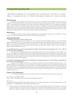
Figure 3 illustrates some of the issues on validation of current generation CTMs against
observational data for the short-lived trace gas, sulphur dioxide (SO2). The figure shows the
annual average model SO2 concentration for the 5 ~ • 5 ~ grid square covering much of England
along with the monthly mean observations for 19 monitoring stations. On this scale, there is
significant spatial variability between the individual measurement sites, which in itself covers
a range of up to a factor of 8. Such a range is likely to be significantly larger than the
uncertainty in emissions. Furthermore, variability is significant at a finer time resolution e.g.
daily or hourly.
The uncertainty in coarse-resolution CTMs operating at 5 ~ x 5 ~ which approximates the
state of the art CTMs, is likely close to a factor of 4 up and down for short-lived trace gases
with significant ecosystem sources and sinks and existing in a complex terrain.
The representation of the trace gas exchange processes in the CTMs at the ecosystem scale
will introduce further uncertainties, the magnitudes of which are crucially dependent on the
nature of the exchange process involved. Dry deposition processes are thought to be the
simplest processes representing the concept of a dry deposition velocity. In this way, many of

the problems of scaling trace gas fluxes can be side-stepped with a simple parameterization.
Clearly, there is a huge gap in scale between the available dry deposition studies on the leaf or
canopy scale and the coarse grid squares of the CTM.
Wet deposition is a sporadic process which is difficult to describe adequately in models.
The coarse spatial resolution of the models is certainly an issue but perhaps more important is
their neglect of the detailed microphysical and chemical processes thought to be occurring in
rain clouds. Simulated global- or regional-scale wet deposition fluxes are available with reaso-
SOa concentration (ppb)
25 25
20 -
15-
10-
5 -
STOCHEM - -+- - Bridge Race - -11( - Lullington Heath
-O- - Ladybower x - Bloomsbun/ -q3- - Birmingham
~ - Sunderland - -0 - Bamsley - -U- - Cardiff 9
~ - Newcastle ~ - Leeds ~ - Bristol t~-
t- Liverpool al$ Birmingham East <) Hull .3'
x- Leicester [3 Southampton ~, Bexley ]r
O Swansea 9 Middlesborough " /
~" I I
N - i
9 ,.',_ .o /t ,x,, x [] o r F'.:, o
9 ~. \ ~ < ]~ ~ . ~ - "/i ".;~:.~"
>*.'-\ ii. ~.0"" " " " 9 '. '" "i" ~ '~
~. .~ x. ~_ ~ .# i
9 ~ .$1~'.'r, .~'. .~: 9
~ ~ .__ ~li
.Ik.^ ~ i~ ~

= '~-:~'~ i-='.C_ ~- ,, ~_
"'_-,m
a:.'~.~-~," -~=~':":'-"~ '='0
,, ~ "~ - .=~ 7- ~_ _ -~ ~
-20
- 15
- 10
-5
0 i I i I I i i I I i I i 0
Jan Feb Mar Apr May Jun Jul Aug Sept Oct Nov Dec
Month
Figure
3. Simulated concentration of SO2 using the STOCHEM model for the 5 x 5 0 grid square covering most
of the U.K. and monthly mean observations for 19 monitoring stations. Source: Stevenson
et al.
(1998).
20
A.F. Bouwman, R.G. Derwent and F.J. Dentener
nable accuracy, but this accuracy deteriorates as spatial scales decrease to the catchment or
landscape scales. Topography is a crucial factor in driving the orographic enhancement of wet
deposition. In coarse-resolution CTMs the topography of all but the highest mountain ranges
is necessarily averaged out, thus removing a major influence on model wet deposition fluxes
to sensitive catchments. There is a consequential reduction in model estimates of cloud water
deposition as the topography is smoothed out by model spatial resolution.
Trace gas exchange with terrestrial and aquatic ecosystems is not always a one-way
process, as emission and resuspension may occur simultaneously (see Conrad and Dentener,
1999). Ammonia emissions are difficult to represent accurately in models because they are
sporadic and depend on local factors, which are highly variable. Soil moisture and animal
husbandry are two such factors which are difficult to be specific about, but which have a
significant influence on ammonia emissions (Bouwman

et al.,
1997). Resuspension of sea-
salts and wind-blown dust is often driven by high winds, which can be adequately represented
in CTMs. However, the state of the terrestrial surfaces, whether wet or recently ploughed, may
have a pronounced influence on resuspension, and these local factors are not often well-
defined on the coarse scales used in the CTMs.
3.3. Comparison of CTMs with emission inventories
With the exception of the spatial resoh".:.on of the emission inventories which meet the
requirements of current CTMs, there are major inconsistencies to remain between the CTMs
and the emission inventories which drive them. The most striking discrepancy between CTMs
and inventories is in the temporal scale, which is generally one year for the inventories and 1-
6 hours for the CTMs. Most CTMs include routines based on hypotheses on temporal flux
distributions at the model scale, or assumptions on temporal patterns are provided with the
emission inventories (see Table 4). Another way is to incorporate the trace gas flux model in
the atmospheric model, as done for example in some CTMs for NOx from soils.
For reactive species with short atmospheric lifetimes such as NH3, NOx and VOC, the
temporal scale gap is a more serious problem than for long-lived species. An additional gap
between inventories and CTMs is the number of VOC species; here, some of the mechanisms
describing the chemistry in CTMs require a much larger number of species than included in
current inventories.
A general major problem is that it is not always possible to ensure that consistent land use
and meteorological data are used throughout the modelling system including the emission
inventorie~. Furthermore, there are scaling problems with all aspects of CTI~ input data, some
of which are caused by limited computer resources, others by the focus of the modelling
system and yet others by lack of current understanding.
Turning to validation of emission inventories, the emission fields for long-lived trace gases
can be tested using CTMs on the basis of concentrations, trends, and seasonality and spatial
gradients of concentrations, as the chemistry is less crucial for long-lived species with fewer
fluctuations over the year. For other species, deposition rates can be used to validate model
results. A discussion of validation tools is, however, outside the scope of this paper. We refer

to Heimann and Kaminski (1999) for a review of inverse modelling and atmospheric
monitoring networks, Trumbore (1999) for a review of the use of isotopes and tracers in
validation and scaling of trace gas fluxes, and to Sofiev (1999) for a discussion on validation
and representativeness of measurement data. A review of the use of remote sensing techniques
to determine atmospheric concentrations is given by Burrows (1999).
Towards reliable global estimates of emissions of trace gases and aerosols 21
4. Conclusions and recommendations
A comparison of the spatial and temporal scales of the present state-of-the-art CTMs and
emission inventories for terrestrial and aquatic ecosystems indicates a wide gap when it comes
to temporal resolution. The most common temporal resolution of emission inventories is one
year, while CTMs describe processes with a time step of 1 to 6 hours. This discrepancy is
particularly" important for gas species with a short atmospheric lifetime (less tt, an one day).
It should be possible to produce estimates for most species and sources with a greater
temporal resolution. However, the key problem involved in increasing the temporal resolution
is the sparsity of data for use as a basis for flux estimates and a lack or even absence of
independent data to validate fluxes. Available data may be appropriate to validate the
temporal variability or the functional relationships between environmental conditions and
fluxes. In general, it becomes increasingly difficult to find tools for validation as the level of
detail of the temporal scale increases. In some cases such data are inadequate or even absent
(e.g. deposition fluxes, concentrations of short-lived species).
The spatial resolution of inventories in our review suggests the level of detail as being
adequate for current CTMs. However, the real spatial resolution of most inventories is much
lower than suggested by the 1 ~ reported. This is caused by the use of emission factors for
biomes and functional types, and by the uncertainty and resolution of the environmental
spatial data used.
The major recommendations following from the examples discussed can be summarized as
follows:
- Emission
factor approaches. Where emissions are described with emission factor or
regression approaches, variability can be used instead of the usual practice of averaging out

the heterogeneity. This is done, for example, by presenting frequency distributions for regions
or functional types, or the standard deviation for grid boxes,. In many cases the point-by-point
uncertainty is not known. However, even the indication of the maximum and minimum values
could be more helpful than the mean alone for sensitivity and quantitative uncertainty
analysis.
- Flux models.
Flux models should be used where possible to replace traditional emission
factor approaches. Firstly, models, which are descriptions of current process knowledge, are
preferred above simple rules such as those applied in CTMs to produce temporal distributions.
Secondly, intemal consistency of CTMs is improved by incorporating the flux models.
In trace-gas flux models there is often an imbalance between the level of detail by which
different processes are described. The relationship between scale, the model approach and the
model parameters selected is very important in this respect. On a higher scale the data
availability, generally poses a problem when using detailed process models. In this case,
simplified or summary models are expected to interpret field experiments with limited
information. The aim of simplifications is to make the model applicable to a wider area with
limited data sets. Developing such ranges of models from the micro-scale to field scale and
summary models to be used for extrapolation to other sites with different conditions is
extremely useful. Summary models will also help to develop a better understanding of how to
select the key variables to be used for specific scales.
- Environmental data.
The spatial data on climate, oceans, soils, land cover and land use
which are commonly used as a basis for scaling of trace fluxes have four general
characteristics: (i) their uncertainty is regionally variable but generally unknown in the spatial
distributions; (ii) data classifications are always aggregations (iii) classifications used are
generally not easily translated into other classifications; (iv) classifications cannot be easily
translated into properties or regulating factors of trace gas fluxes. In view of these
22
A.F. Bouwman, R. G. Derwent and F.J. Dentener
characteristics the use of common databases should be promoted.

Geographic databases coupled with attribute files for the various map units distinguished is
one way to at least describe the heterogeneity of the properties within a class. Examples of this
approach are the soil database and the land-cover characterization discussed in this paper.
Combining vegetation/land-cover data with climate and soil information may provide a basis
for classification according to function. Finally, there is a need for compensation and
recognition of so-called data collectors to encourage continued critical data collection,
harmonization and analysis.
- Functional
types. Where distinct and easily identified differences in structure and
composition of aquatic and terrestrial ecosystems coincide with the functions or management
conditions relevant to trace-gas fluxes at the scale considered, the delineation of functionally
different types or production/management systems provides a useful basis both for
measurement strategies and scaling. Appropriate selection of classes may lead to reducing the
number of sites to be sampled so as to derive a reliable flux estimate. Maps provide a useful
basis for delineation, and in recent years remote sensing of ecosystem characteristics has been
used increasingly for classification and modelling (see Estes and Loveland, 1999). Such
approaches use the variability of a system or landscape instead of ignoring it, sometimes with
unexpected consequences. It is very important to select appropriate stratification schemes for
functional types, both for the scale of the exercise and the available spatial data.
- Aggregation. Aggregation always leads to a loss of information. The variability in space is
reduced and the uncertainty in the temporal patterns is increased by spatial aggregations. The
problem of errors in temporal distributions as a result of spatial aggregation can be reduced by
delineating functional types within a system. Scaling based on delineations with finer spatial
data may be different from that derived from data with lower resolution. In general, it is better to
aggregate model results than to aggregate the spatial data before modelling. Aggregation in the
form of delineation of functional types as a basis for scaling generally decreases the
uncertainty, and allows one to determine the uncertainties as discussed above.
- Interannuai
variability. Some processes in terrestrial and aquatic ecosystems show con-
siderable year-to-year variation. Hence, in such systems with large interannual variability, in-

ventories representing the long-range average have less value than time series of flux
estimates.
This paper has reviewed the uncertainties in estimating emissions from land-use-related,
and natural terrestrial and aquatic sources. A comparison has also been drawn up between the
available inventories and the requirements of state-of-the-art CTMs. We have shown a
number of weaknesses and problems in current methods for estimating emissions. We have
also presented several possibilities for improving flux estimates, hoping that these
recommendations will stimulate further study and discussion on the reduction of uncertainties
in flux estimates.
References
Allen, D.J., P. Kasibhatla, A.M. Thompson, R.B. Rood, B.G. Doddridge, K.E. Pickering, R.D.
Hudson and S-J. Lin (1996) Transport-induced interannual variability of carbon monoxide
determined using a chemistry and transport model. Journal of Geophysical Research 101:28655-
28669.
Andreae, M.O. (1991) Biomass burning: its history, use and distribution and its impact on environmental
quality and global climate. In: Levine, J.S. (Ed.) Global Biomass Burning. MIT Press, Cambridge, pp.
3-28.
Towards reliable global estimates of emissions of trace gases and aerosols 23
Asman, W.A.H. (1992) Ammonia emission in Europe: updated emission and emission variations. Report
228471008, National Institute of Public Health and the Environment, Bilthoven, Netherlands.
Batjes, N.H. (1996) Total carbon and nitrogen in the soils of the world. European Journal of Soil
Science 47:151-163.
Batjes, N.H. (1997) A world data set of derived soil properties by FAO-Unesco soil unit for global
modelling. Soil Use and Management 13:9-16.
Batjes, N.H. and E.M. Bridges (1994) Potential emissions of radiatively active gases from soil to
atmosphere with special reference to methane: development of a global database (WISE). Journal
of Geop.hysical Research 99:16479-16489:
Benkovitz, C.M. and M.A. Mubaraki (1996) Sulfur emissions from volcanic activity in 1985 and
1990. In: A.S. Lefohn, J.D. Husar and R.B. Husar (Eds.) Assessing historical global sulfur
emission patterns for the period 1850 and 1990. US Department of Energy, Washington DC, pp.

C1-C18.
Bernsten T., I.S.A. Isaksen, W-C. Wang and X Z. Liang (1996) Impacts of increased anthropogenic
emissions in Asia on tropospheric ozone and climate. Tellus 45B: 13-32.
Bouwman, A.F. and J.A. Taylor (1996) Testing high-resolution nitrous oxide emission estimates
against observations using an atmospheric transport model. Global Biogeochemical Cycles 10:307-
318.
Bouwman, A.F., I. Fung, E. Matthews and J. John (1993) Global analysis of the potential for N20
production in natural soils. Global Biogeochemical Cycles 7:557-597.
Bouwman, A.F., D.S. Lee, W.A.H. Asman, F.J. Dentener, K.W. van der Hoek and J.G.J. Olivier
(1997) A global high-resolution emission inventory for ammonia. Global Biogeochemical Cycles
11:561-587.
Brasseur, G.P., D.A. Hauglustaine, C. Granier, J F. Muller, P. Rasch, X.X. Tie and S. Walters (1997)
MOZART: A global three-dimensional chemical-transport model of the atmosphere. Journal of
Geophysical Research (in press).
Burrows, J.P. (1999) Current and future passive remote sensing techniques used to determine
atmospheric constituents. In: A.F. Bouwman (Ed.) Approaches to scaling of trace gas fluxes in
ecosystems. Developments in Atmospheric Science 24. Elsevier, Amsterdam, pp. 313-347.
Chin, M., D.J. Jacob, G.M. Gardner, Foreman-Fowler and P. Spiro (1996) A global three-dimensional
model of tropospheric sulphate. Journal of Geophysical Research 101:18667-18690.
Collins, W.J., D.S. Stevenson, C.E. Johnson and R.G. Derwent (1997) Tropospheric ozone in a
global-scale three-dimensional Lagrangian model and its response to NOx controls. Journal of
Atmospheric Chemistry 26:223-274.
Conkright, M., S. Levitus and T. Boyer (1994) Worm Ocean Atlas 1994, Volume 1." Nutrients. NOAA
Atlas NESDIS 1, US Department of Commerce, Washington, DC.
Conrad, R. and F. Dentener (1999) The application of the compensation point concepts in scaling of
fluxes. In: A.F. Bouwman (Ed.) Approaches to scaling of trace gas fluxes in ecosystems.
Developments in Atmospheric Science 24. Elsevier, Amsterdam, pp. 203-216
Cramer, W. and A. Fischer (1996) Data requirements for terrestrial ecosystem modelling. In: B.
Walker and W. Steffen (Eds.) Global change and terrestrial ecosystems, International Geosphere-
Biosphere programme Book Series, Cambridge University Press, Cambridge UK, pp. 529-565.

Davidson, E.A. and W. Kingerlee (1997) A global inventory of nitric oxide emissions from soils.
Nutrient Cycling in Agroecosystems 48:37-50.
Denmead, O.T., R. Leuning, D.W.T. Griffith and C.P. Meyer (1999) Some recent developments in
trace gas flux measurement. In: A.F. Bouwman (Ed.) Approaches to scaling of trace gas fluxes in
ecosystems. Developments in Atmospheric Science 24. Elsevier, Amsterdam, pp. 67-84.
Dentener F.J. and P.J. Crutzen (1993) Reaction of N205 on tropospheric aerosols: Impact on the
global distributions of NOx, 03 and OH. Journal of Geophysical Research 98:7149-7163.
EEA (1997) Corinair 94 summary report. European Topic Centre on Air Emissions. Report to the
European Environment Agency, I20 pp.
EPA (1993) Regional interim emission inventories (1987-1991) Report 454/R-93-021, U.S.
Environmental Protection Agency, Research Triangle Park.