A SURVEY OF BEHAVIORAL FINANCE° pot
Bạn đang xem bản rút gọn của tài liệu. Xem và tải ngay bản đầy đủ của tài liệu tại đây (291.6 KB, 71 trang )
Chapter 18
A SURVEY OF BEHAVIORAL FINANCE
°
NICHOLAS BARBERIS
University of Chicago
RICHARD THALER
University of Chicago
Contents
Abstract 1052
Keywords 1052
1. Introduction 1053
2. Limits to arbitrage 1054
2.1. Market efficiency 1054
2.2. Theory 1056
2.3. Evidence 1059
2.3.1. Twin shares 1059
2.3.2. Index inclusions 1061
2.3.3. Internet carve-outs 1062
3. Psychology 1063
3.1. Beliefs 1063
3.2. Preferences 1067
3.2.1. Prospect theory 1067
3.2.2. Ambiguity aversion 1072
4. Application: The aggregate stock market 1073
4.1. The equity premium puzzle 1076
4.1.1. Prospect theory 1077
4.1.2. Ambiguity aversion 1080
4.2. The volatility puzzle 1081
4.2.1. Beliefs 1082
4.2.2. Preferences 1084
5. Application: The cross-section of average returns 1085
5.1. Belief-based models 1090
°
We are very grateful to Markus Brunnermeier, George Constantinides, Kent Daniel, Milt Harris, Ming
Huang, Owen Lamont, Jay Ritter, Andrei Shleifer, Jeremy Stein and Tuomo Vuolteenaho for extensive
comments.
Handbook of the Economics of Finance, Edited by G.M. Constantinides, M. Harris and R. Stulz
© 2003 Elsevier Science B.V. All rights reserved
1052 N. Barberis and R. Thaler
5.2. Belief-based models with institutional frictions
1093
5.3. Preferences 1095
6. Application: Closed-end funds and comovement 1096
6.1. Closed-end funds 1096
6.2. Comovement 1097
7. Application: Investor behavior 1099
7.1. Insufficient diversification 1099
7.2. Naive diversification 1101
7.3. Excessive trading 1101
7.4. The selling decision 1102
7.5. The buying decision 1103
8. Application: Corporate finance 1104
8.1. Security issuance, capital structure and investment 1104
8.2. Dividends
1107
8.3. Models of managerial irrationality 1109
9. Conclusion 1111
Appendix A 1113
References 1114
Abstract
Behavioral finance argues that some financial phenomena can plausibly be understood
using models in which some agents are not fully rational. The field has two building
blocks: limits to arbitrage, which argues that it can be difficult for rational traders to
undo the dislocations caused by less rational traders; and psychology, which catalogues
the kinds of deviations from full rationality we might expect to see. We discuss
these two topics, and then present a number of behavioral finance applications: to the
aggregate stock market, to the cross-section of average returns, to individual trading
behavior, and to corporate finance. We close by assessing progress in the field and
speculating about its future course.
Keywords
behavioral finance, market efficiency, prospect theory, limits to arbitrage, investor
psychology, investor behavior
JEL classification: G11, G12, G30
Ch. 18: A Survey of Behavioral Finance 1053
1. Introduction
The traditional finance paradigm, which underlies many of the other articles in this
handbook, seeks to understand financial markets using models in which agents are
“rational”. Rationality means two things. First, when they receive new information,
agents update their beliefs correctly, in the manner described by Bayes’ law. Second,
given their beliefs, agents make choices that are normatively acceptable, in the sense
that they are consistent with Savage’s notion of Subjective Expected Utility (SEU).
This traditional framework is appealingly simple, and it would be very satisfying
if its predictions were confirmed in the data. Unfortunately, after years of effort, it
has become clear that basic facts about the aggregate stock market, the cross-section
of average returns and individual trading behavior are not easily understood in this
framework.
Behavioral finance is a new approach to financial markets that has emerged, at least
in part, in response to the difficulties faced by the traditional paradigm. In broad terms,
it argues that some financial phenomena can be better understood using models in
which some agents are not fully rational. More specifically, it analyzes what happens
when we relax one, or both, of the two tenets that underlie individual rationality.
In some behavioral finance models, agents fail to update their beliefs correctly. In
other models, agents apply Bayes’ law properly but make choices that are normatively
questionable, in that they are incompatible with SEU.
1
This review essay evaluates recent work in this rapidly growing field. In Section 2,
we consider the classic objection to behavioral finance, namely that even if some agents
in the economy are less than fully rational, rational agents will prevent them from
influencing security prices for very long, through a process known as arbitrage. One
of the biggest successes of behavioral finance is a series of theoretical papers showing
that in an economy where rational and irrational traders interact, irrationality can have
a substantial and long-lived impact on prices. These papers, known as the literature
on “limits to arbitrage”, form one of the two buildings blocks of behavioral finance.
1
It is important to note that most models of asset pricing use the Rational Expectations Equilibrium
framework (REE), which assumes not only individual rationality but also consistent beliefs [Sargent
(1993)]. Consistent beliefs means that agents’ beliefs are correct: the subjective distribution they use
to forecast future realizations of unknown variables is indeed the distribution that those realizations are
drawn from. This requires not only that agents process new information correctly, but that they have
enough information about the structure of the economy to be able to figure out the correct distribution
for the variables of interest.
Behavioral finance departs from REE by relaxing the assumption of individual rationality. An
alternative departure is to retain individual rationality but to relax the consistent beliefs assumption: while
investors apply Bayes’ law correctly, they lack the information required to know the actual distribution
variables are drawn from. This line of research is sometimes referred to as the literature on bounded
rationality, or on structural uncertainty. For example, a model in which investors do not know the growth
rate of an asset’s cash flows but learn it as best as they can from available data, would fall into this
class. Although the literature we discuss also uses the term bounded rationality, the approach is quite
different.
1054 N. Barberis and R. Thaler
To make sharp predictions, behavioral models often need to specify the form of
agents’ irrationality. How exactly do people misapply Bayes law or deviate from
SEU? For guidance on this, behavioral economists typically turn to the extensive
experimental evidence compiled by cognitive psychologists on the biases that arise
when people form beliefs, and on people’s preferences, or on how they make decisions,
given their beliefs. Psychology is therefore the second building block of behavioral
finance, and we review the psychology most relevant for financial economists in
Section 3.
2
In Sections 4–8, we consider specific applications of behavioral finance: to
understanding the aggregate stock market, the cross-section of average returns, and the
pricing of closed-end funds in Sections 4, 5 and 6 respectively; to understanding how
particular groups of investors choose their portfolios and trade over time in Section 7;
and to understanding the financing and investment decisions of firms in Section 8.
Section 9 takes stock and suggests directions for future research.
3
2. Limits to arbitrage
2.1. Market efficiency
In the traditional framework where agents are rational and there are no frictions,
a security’s price equals its “fundamental value”. This is the discounted sum
of expected future cash flows, where in forming expectations, investors correctly
process all available information, and where the discount rate is consistent with a
normatively acceptable preference specification. The hypothesis that actual prices
reflect fundamental values is the Efficient Markets Hypothesis (EMH). Put simply,
under this hypothesis, “prices are right”, in that they are set by agents who understand
Bayes’ law and have sensible preferences. In an efficient market, there is “no free
lunch”: no investment strategy can earn excess risk-adjusted average returns, or average
returns greater than are warranted for its risk.
Behavioral finance argues that some features of asset prices are most plausibly
interpreted as deviations from fundamental value, and that these deviations are brought
about by the presence of traders who are not fully rational. A long-standing objection
to this view that goes back to Friedman (1953) is that rational traders will quickly
undo any dislocations caused by irrational traders. To illustrate the argument, suppose
2
The idea, now widely adopted, that behavioral finance rests on the two pillars of limits to arbitrage
and investor psychology is originally due to Shleifer and Summers (1990).
3
We draw readers’ attention to two other recent surveys of behavioral finance. Shleifer (2000) provides
a particularly detailed discussion of the theoretical and empirical work on limits to arbitrage, which
we summarize in Section 2. Hirshleifer’s (2001) survey is closer to ours in terms of material covered,
although we devote less space to asset pricing, and more to corporate finance and individual investor
behavior. We also organize the material somewhat differently.
Ch. 18: A Survey of Behavioral Finance 1055
that the fundamental value of a share of Ford is $20. Imagine that a group of irrational
traders becomes excessively pessimistic about Ford’s future prospects and through its
selling, pushes the price to $15. Defenders of the EMH argue that rational traders,
sensing an attractive opportunity, will buy the security at its bargain price and at the
same time, hedge their bet by shorting a “substitute” security, such as General Motors,
that has similar cash flows to Ford in future states of the world. The buying pressure
on Ford shares will then bring their price back to fundamental value.
Friedman’s line of argument is initially compelling, but it has not survived careful
theoretical scrutiny. In essence, it is based on two assertions. First, as soon as
there is a deviation from fundamental value – in short, a mispricing – an attractive
investment opportunity is created. Second, rational traders will immediately snap up
the opportunity, thereby correcting the mispricing. Behavioral finance does not take
issue with the second step in this argument: when attractive investment opportunities
come to light, it is hard to believe that they are not quickly exploited. Rather, it disputes
the first step. The argument, which we elaborate on in Sections 2.2 and 2.3, is that even
when an asset is wildly mispriced, strategies designed to correct the mispricing can
be both risky and costly, rendering them unattractive. As a result, the mispricing can
remain unchallenged.
It is interesting to think about common finance terminology in this light. While
irrational traders are often known as “noise traders”, rational traders are typically
referred to as “arbitrageurs”. Strictly speaking, an arbitrage is an investment strategy
that offers riskless profits at no cost. Presumably, the rational traders in Friedman’s
fable became known as arbitrageurs because of the belief that a mispriced asset
immediately creates an opportunity for riskless profits. Behavioral finance argues that
this is not true: the strategies that Friedman would have his rational traders adopt are
not necessarily arbitrages; quite often, they are very risky.
An immediate corollary of this line of thinking is that “prices are right” and “there
is no free lunch” are not equivalent statements. While both are true in an efficient
market, “no free lunch” can also be true in an inefficient market: just because prices
are away from fundamental value does not necessarily mean that there are any excess
risk-adjusted average returns for the taking. In other words,
“prices are right” ⇒ “no free lunch”
but
“no free lunch” “prices are right”.
This distinction is important for evaluating the ongoing debate on market efficiency.
First, many researchers still point to the inability of professional money managers
to beat the market as strong evidence of market efficiency [Rubinstein (2001), Ross
(2001)]. Underlying this argument, though, is the assumption that “no free lunch”
implies “prices are right.” If, as we argue in Sections 2.2 and 2.3, this link is broken, the
1056 N. Barberis and R. Thaler
performance of money managers tells us little about whether prices reflect fundamental
value.
Second, while some researchers accept that there is a distinction between “prices
are right” and “there is no free lunch”, they believe that the debate should be more
about the latter statement than about the former. We disagree with this emphasis. As
economists, our ultimate concern is that capital be allocated to the most promising
investment opportunities. Whether this is true or not depends much more on whether
prices are right than on whether there are any free lunches for the taking.
2.2. Theory
In the previous section, we emphasized the idea that when a mispricing occurs,
strategies designed to correct it can be both risky and costly, thereby allowing the
mispricing to survive. Here we discuss some of the risks and costs that have been
identified. In our discussion, we return to the example of Ford, whose fundamental
value is $20, but which has been pushed down to $15 by pessimistic noise traders.
Fundamental risk. The most obvious risk an arbitrageur faces if he buys Ford’s stock
at $15 is that a piece of bad news about Ford’s fundamental value causes the stock to
fall further, leading to losses. Of course, arbitrageurs are well aware of this risk, which
is why they short a substitute security such as General Motors at the same time that
they buy Ford. The problem is that substitute securities are rarely perfect, and often
highly imperfect, making it impossible to remove all the fundamental risk. Shorting
General Motors protects the arbitrageur somewhat from adverse news about the car
industry as a whole, but still leaves him vulnerable to news that is specific to Ford –
news about defective tires, say.
4
Noise trader risk. Noise trader risk, an idea introduced by De Long et al. (1990a)
and studied further by Shleifer and Vishny (1997), is the risk that the mispricing
being exploited by the arbitrageur worsens in the short run. Even if General Motors
is a perfect substitute security for Ford, the arbitrageur still faces the risk that the
pessimistic investors causing Ford to be undervalued in the first place become even
more pessimistic, lowering its price even further. Once one has granted the possibility
that a security’s price can be different from its fundamental value, then one must also
grant the possibility that future price movements will increase the divergence.
Noise trader risk matters because it can force arbitrageurs to liquidate their positions
early, bringing them potentially steep losses. To see this, note that most real-world
arbitrageurs – in other words, professional portfolio managers – are not managing their
4
Another problem is that even if a substitute security exists, it may itself be mispriced. This can happen
in situations involving industry-wide mispricing: in that case, the only stocks with similar future cash
flows to the mispriced one are themselves mispriced.
Ch. 18: A Survey of Behavioral Finance 1057
own money, but rather managing money for other people. In the words of Shleifer and
Vishny (1997), there is “a separation of brains and capital”.
This agency feature has important consequences. Investors, lacking the specialized
knowledge to evaluate the arbitrageur’s strategy, may simply evaluate him based on
his returns. If a mispricing that the arbitrageur is trying to exploit worsens in the
short run, generating negative returns, investors may decide that he is incompetent,
and withdraw their funds. If this happens, the arbitrageur will be forced to liquidate
his position prematurely. Fear of such premature liquidation makes him less aggressive
in combating the mispricing in the first place.
These problems can be severely exacerbated by creditors. After poor short-term
returns, creditors, seeing the value of their collateral erode, will call their loans, again
triggering premature liquidation.
In these scenarios, the forced liquidation is brought about by the worsening of the
mispricing itself. This need not always be the case. For example, in their efforts to
remove fundamental risk, many arbitrageurs sell securities short. Should the original
owner of the borrowed security want it back, the arbitrageur may again be forced to
close out his position if he cannot find other shares to borrow. The risk that this occurs
during a temporary worsening of the mispricing makes the arbitrageur more cautious
from the start.
Implementation costs. Well-understood transaction costs such as commissions, bid–
ask spreads and price impact can make it less attractive to exploit a mispricing.
Since shorting is often essential to the arbitrage process, we also include short-sale
constraints in the implementation costs category. These refer to anything that makes it
less attractive to establish a short position than a long one. The simplest such constraint
is the fee charged for borrowing a stock. In general these fees are small – D’Avolio
(2002) finds that for most stocks, they range between 10 and 15 basis points – but
they can be much larger; in some cases, arbitrageurs may not be able to find shares to
borrow at any price. Other than the fees themselves, there can be legal constraints: for
a large fraction of money managers – many pension fund and mutual fund managers
in particular – short-selling is simply not allowed.
5
We also include in this category the cost of finding and learning about a mispricing,
as well as the cost of the resources needed to exploit it [Merton (1987)]. Finding
5
The presence of per-period transaction costs like lending fees can expose arbitrageurs to another kind
of risk, horizon risk, which is the risk that the mispricing takes so long to close that any profits are
swamped by the accumulated transaction costs. This applies even when the arbitrageur is certain that
no outside party will force him to liquidate early. Abreu and Brunnermeier (2002) study a particular
type of horizon risk, which they label synchronization risk. Suppose that the elimination of a mispricing
requires the participation of a sufficiently large number of separate arbitrageurs. Then in the presence
of per-period transaction costs, arbitrageurs may hesitate to exploit the mispricing because they don’t
know how many other arbitrageurs have heard about the opportunity, and therefore how long they will
have to wait before prices revert to correct values.
1058 N. Barberis and R. Thaler
mispricing, in particular, can be a tricky matter. It was once thought that if noise
traders influenced stock prices to any substantial degree, their actions would quickly
show up in the form of predictability in returns. Shiller (1984) and Summers (1986)
demonstrate that this argument is completely erroneous, with Shiller (1984) calling
it “one of the most remarkable errors in the history of economic thought”. They
show that even if noise trader demand is so strong as to cause a large and persistent
mispricing, it may generate so little predictability in returns as to be virtually
undetectable.
In contrast, then, to straightforward-sounding textbook arbitrage, real world arbitrage
entails both costs and risks, which under some conditions will limit arbitrage and allow
deviations from fundamental value to persist. To see what these conditions are, consider
two cases.
Suppose first that the mispriced security does not have a close substitute. By
definition then, the arbitrageur is exposed to fundamental risk. In this case, sufficient
conditions for arbitrage to be limited are (i) that arbitrageurs are risk averse and (ii) that
the fundamental risk is systematic, in that it cannot be diversified by taking many
such positions. Condition (i) ensures that the mispricing will not be wiped out by
a single arbitrageur taking a large position in the mispriced security. Condition (ii)
ensures that the mispricing will not be wiped out by a large number of investors
each adding a small position in the mispriced security to their current holdings.
The presence of noise trader risk or implementation costs will only limit arbitrage
further.
Even if a perfect substitute does exist, arbitrage can still be limited. The existence
of the substitute security immunizes the arbitrageur from fundamental risk. We can go
further and assume that there are no implementation costs, so that only noise trader risk
remains. De Long et al. (1990a) show that noise trader risk is powerful enough, that
even with this single form of risk, arbitrage can sometimes be limited. The sufficient
conditions are similar to those above, with one important difference. Here arbitrage
will be limited if: (i) arbitrageurs are risk averse and have short horizons and (ii) the
noise trader risk is systematic. As before, condition (i) ensures that the mispricing
cannot be wiped out by a single, large arbitrageur, while condition (ii) prevents a large
number of small investors from exploiting the mispricing. The central contribution of
Shleifer and Vishny (1997) is to point out the real world relevance of condition (i):
the possibility of an early, forced liquidation means that many arbitrageurs effectively
have short horizons.
In the presence of certain implementation costs, condition (ii) may not even be
necessary. If it is costly to learn about a mispricing, or the resources required to
exploit it are expensive, that may be enough to explain why a large number of different
individuals do not intervene in an attempt to correct the mispricing.
It is also important to note that for particular types of noise trading, arbitrageurs
may prefer to trade in the same direction as the noise traders, thereby exacerbating
the mispricing, rather than against them. For example, De Long et al. (1990b)
Ch. 18: A Survey of Behavioral Finance 1059
consider an economy with positive feedback traders, who buy more of an asset this
period if it performed well last period. If these noise traders push an asset’s price
above fundamental value, arbitrageurs do not sell or short the asset. Rather, they
buy it, knowing that the earlier price rise will attract more feedback traders next
period, leading to still higher prices, at which point the arbitrageurs can exit at a
profit.
So far, we have argued that it is not easy for arbitrageurs like hedge funds to exploit
market inefficiencies. However, hedge funds are not the only market participants trying
to take advantage of noise traders: firm managers also play this game. If a manager
believes that investors are overvaluing his firm’s shares, he can benefit the firm’s
existing shareholders by issuing extra shares at attractive prices. The extra supply this
generates could potentially push prices back to fundamental value.
Unfortunately, this game entails risks and costs for managers, just as it does for
hedge funds. Issuing shares is an expensive process, both in terms of underwriting
fees and time spent by company management. Moreover, the manager can rarely be
sure that investors are overvaluing his firm’s shares. If he issues shares, thinking that
they are overvalued when in fact they are not, he incurs the costs of deviating from
his target capital structure, without getting any benefits in return.
2.3. Evidence
From the theoretical point of view, there is reason to believe that arbitrage is a
risky process and therefore that it is only of limited effectiveness. But is there any
evidence that arbitrage is limited? In principle, any example of persistent mispricing
is immediate evidence of limited arbitrage: if arbitrage were not limited, the mispricing
would quickly disappear. The problem is that while many pricing phenomena can be
interpreted as deviations from fundamental value, it is only in a few cases that the
presence of a mispricing can be established beyond any reasonable doubt. The reason
for this is what Fama (1970) dubbed the “joint hypothesis problem”. In order to claim
that the price of a security differs from its properly discounted future cash flows, one
needs a model of “proper” discounting. Any test of mispricing is therefore inevitably a
joint test of mispricing and of a model of discount rates, making it difficult to provide
definitive evidence of inefficiency.
In spite of this difficulty, researchers have uncovered a number of financial
market phenomena that are almost certainly mispricings, and persistent ones at that.
These examples show that arbitrage is indeed limited, and also serve as interesting
illustrations of the risks and costs described earlier.
2.3.1. Twin shares
In 1907, Royal Dutch and Shell Transport, at the time completely independent
companies, agreed to merge their interests on a 60:40 basis while remaining separate
entities. Shares of Royal Dutch, which are primarily traded in the USA and in the
1060 N. Barberis and R. Thaler
Fig. 1. Log deviations from Royal Dutch/Shell parity. Source: Froot and Dabora (1999).
Netherlands, are a claim to 60% of the total cash flow of the two companies, while
Shell, which trades primarily in the UK, is a claim to the remaining 40%. If prices
equal fundamental value, the market value of Royal Dutch equity should always be
1.5 times the market value of Shell equity. Remarkably, it isn’t.
Figure 1, taken from Froot and Dabora’s (1999) analysis of this case, shows the ratio
of Royal Dutch equity value to Shell equity value relative to the efficient markets
benchmark of 1.5. The picture provides strong evidence of a persistent inefficiency.
Moreover, the deviations are not small. Royal Dutch is sometimes 35% underpriced
relative to parity, and sometimes 15% overpriced.
This evidence of mispricing is simultaneously evidence of limited arbitrage, and it is
not hard to see why arbitrage might be limited in this case. If an arbitrageur wanted to
exploit this phenomenon – and several hedge funds, Long-Term Capital Management
included, did try to – he would buy the relatively undervalued share and short the
other. Table 1 summarizes the risks facing the arbitrageur. Since one share is a good
substitute for the other, fundamental risk is nicely hedged: news about fundamentals
should affect the two shares equally, leaving the arbitrageur immune. Nor are there
Table 1
Arbitrage costs and risks that arise in exploiting mispricing
Example Fundamental
risk (FR)
Noise
trader risk (NTR)
Implementation
costs (IC)
Royal Dutch/Shell ×
√
×
Index Inclusions
√√
×
Palm/3Com ××
√
Ch. 18: A Survey of Behavioral Finance 1061
any major implementation costs to speak of: shorting shares of either company is an
easy matter.
The one risk that remains is noise trader risk. Whatever investor sentiment is causing
one share to be undervalued relative to the other could also cause that share to become
even more undervalued in the short term. The graph shows that this danger is very
real: an arbitrageur buying a 10% undervalued Royal Dutch share in March 1983 would
have seen it drop still further in value over the next six months. As discussed earlier,
when a mispriced security has a perfect substitute, arbitrage can still be limited if
(i) arbitrageurs are risk averse and have short horizons and (ii) the noise trader risk is
systematic, or the arbitrage requires specialized skills, or there are costs to learning
about such opportunities. It is very plausible that both (i) and (ii) are true, thereby
explaining why the mispricing persisted for so long. It took until 2001 for the shares
to finally sell at par.
This example also provides a nice illustration of the distinction between “prices are
right” and “no free lunch” discussed in Section 2.1. While prices in this case are clearly
not right, there are no easy profits for the taking.
2.3.2. Index inclusions
Every so often, one of the companies in the S&P 500 is taken out of the index because
of a merger or bankruptcy, and is replaced by another firm. Two early studies of such
index inclusions, Harris and Gurel (1986) and Shleifer (1986), document a remarkable
fact: when a stock is added to the index, it jumps in price by an average of 3.5%, and
much of this jump is permanent. In one dramatic illustration of this phenomenon, when
Yahoo was added to the index, its shares jumped by 24% in a single day.
The fact that a stock jumps in value upon inclusion is once again clear evidence
of mispricing: the price of the share changes even though its fundamental value does
not. Standard and Poor’s emphasizes that in selecting stocks for inclusion, they are
simply trying to make their index representative of the U.S. economy, not to convey
any information about the level or riskiness of a firm’s future cash flows.
6
This example of a deviation from fundamental value is also evidence of limited
arbitrage. When one thinks about the risks involved in trying to exploit the anomaly,
its persistence becomes less surprising. An arbitrageur needs to short the included
security and to buy as good a substitute security as he can. This entails considerable
6
After the initial studies on index inclusions appeared, some researchers argued that the price increase
might be rationally explained through information or liquidity effects. While such explanations cannot
be completely ruled out, the case for mispricing was considerably strengthened by Kaul, Mehrotra
and Morck (2000). They consider the case of the TS300 index of Canadian equities, which in 1996
changed the weights of some of its component stocks to meet an innocuous regulatory requirement. The
reweighting was accompanied by significant price effects. Since the affected stocks were already in the
index at the time of the event, information and liquidity explanations for the price jumps are extremely
implausible.
1062 N. Barberis and R. Thaler
fundamental risk because individual stocks rarely have good substitutes. It also carries
substantial noise trader risk: whatever caused the initial jump in price – in all
likelihood, buying by S&P 500 index funds – may continue, and cause the price to rise
still further in the short run; indeed, Yahoo went from $115 prior to its S&P inclusion
announcement to $210 a month later.
Wurgler and Zhuravskaya (2002) provide additional support for the limited arbitrage
view of S&P 500 inclusions. They hypothesize that the jump upon inclusion should be
particularly large for those stocks with the worst substitute securities, in other words,
for those stocks for which the arbitrage is riskiest. By constructing the best possible
substitute portfolio for each included stock, they are able to test this, and find strong
support. Their analysis also shows just how hard it is to find good substitute securities
for individual stocks. For most regressions of included stock returns on the returns of
the best substitute securities, the R
2
is below 25%.
2.3.3. Internet carve-outs
In March 2000, 3Com sold 5% of its wholly owned subsidiary Palm Inc. in an initial
public offering, retaining ownership of the remaining 95%. After the IPO, a shareholder
of 3Com indirectly owned 1.5 shares of Palm. 3Com also announced its intention to
spin off the remainder of Palm within 9 months, at which time they would give each
3Com shareholder 1.5 shares of Palm.
At the close of trading on the first day after the IPO, Palm shares stood at $95,
putting a lower bound on the value of 3Com at $142. In fact, 3Com’s price was $81,
implying a market valuation of 3Com’s substantial businesses outside of Palm of about
−$60 per share!
This situation surely represents a severe mispricing, and it persisted for several
weeks. To exploit it, an arbitrageur could buy one share of 3Com, short 1.5 shares
of Palm, and wait for the spin-off, thus earning certain profits at no cost. This strategy
entails no fundamental risk and no noise trader risk. Why, then, is arbitrage limited?
Lamont and Thaler (2003), who analyze this case in detail, argue that implementation
costs played a major role. Many investors who tried to borrow Palm shares to short
were either told by their broker that no shares were available, or else were quoted a
very high borrowing price. This barrier to shorting was not a legal one, but one that
arose endogenously in the marketplace: such was the demand for shorting Palm, that
the supply of Palm shorts was unable to meet it. Arbitrage was therefore limited, and
the mispricing persisted.
7
Some financial economists react to these examples by arguing that they are simply
isolated instances with little broad relevance.
8
We think this is an overly complacent
7
See also Mitchell, Pulvino and Stafford (2002) and Ofek and Richardson (2003) for further discussion
of such “negative stub” situations, in which the market value of a company is less than the sum of its
publicly traded parts.
8
During a discussion of these issues at a University of Chicago seminar, one economist argued that
these examples are “the tip of the iceberg”, to which another retorted that “they are the iceberg”.
Ch. 18: A Survey of Behavioral Finance 1063
view. The “twin shares” example illustrates that in situations where arbitrageurs
face only one type of risk – noise trader risk – securities can become mispriced
by almost 35%. This suggests that if a typical stock trading on the NYSE or
NASDAQ becomes subject to investor sentiment, the mispricing could be an order
of magnitude larger. Not only would arbitrageurs face noise trader risk in trying to
correct the mispricing, but fundamental risk as well, not to mention implementation
costs.
3. Psychology
The theory of limited arbitrage shows that if irrational traders cause deviations from
fundamental value, rational traders will often be powerless to do anything about it.
In order to say more about the structure of these deviations, behavioral models often
assume a specific form of irrationality. For guidance on this, economists turn to the
extensive experimental evidence compiled by cognitive psychologists on the systematic
biases that arise when people form beliefs, and on people’s preferences.
9
In this section, we summarize the psychology that may be of particular interest to
financial economists. Our discussion of each finding is necessarily brief. For a deeper
understanding of the phenomena we touch on, we refer the reader to the surveys of
Camerer (1995) and Rabin (1998) and to the edited volumes of Kahneman, Slovic and
Tversky (1982), Kahneman and Tversky (2000) and Gilovich, Griffin and Kahneman
(2002).
3.1. Beliefs
A crucial component of any model of financial markets is a specification of how agents
form expectations. We now summarize what psychologists have learned about how
people appear to form beliefs in practice.
Overconfidence. Extensive evidence shows that people are overconfident in their
judgments. This appears in two guises. First, the confidence intervals people assign
to their estimates of quantities – the level of the Dow in a year, say – are far too
narrow. Their 98% confidence intervals, for example, include the true quantity only
about 60% of the time [Alpert and Raiffa (1982)]. Second, people are poorly calibrated
when estimating probabilities: events they think are certain to occur actually occur only
9
We emphasize, however, that behavioral models do not need to make extensive psychological
assumptions in order to generate testable predictions. In Section 6, we discuss Lee, Shleifer and Thaler’s
(1991) theory of closed-end fund pricing. That theory makes numerous crisp predictions using only the
assumptions that there are noise traders with correlated sentiment in the economy, and that arbitrage is
limited.
1064 N. Barberis and R. Thaler
around 80% of the time, and events they deem impossible occur approximately 20%
of the time [Fischhoff, Slovic and Lichtenstein (1977)].
10
Optimism and wishful thinking. Most people display unrealistically rosy views of
their abilities and prospects [Weinstein (1980)]. Typically, over 90% of those surveyed
think they are above average in such domains as driving skill, ability to get along
with people and sense of humor. They also display a systematic planning fallacy: they
predict that tasks (such as writing survey papers) will be completed much sooner than
they actually are [Buehler, Griffin and Ross (1994)].
Representativeness. Kahneman and Tversky (1974) show that when people try to
determine the probability that a data set A was generated by a model B, or that an
object A belongs to a class B, they often use the representativeness heuristic. This
means that they evaluate the probability by the degree to which A reflects the essential
characteristics of B.
Much of the time, representativeness is a helpful heuristic, but it can generate some
severe biases. The first is base rate neglect. To illustrate, Kahneman and Tversky
present this description of a person named Linda:
Linda is 31 years old, single, outspoken, and very bright. She majored in philosophy.
As a student, she was deeply concerned with issues of discrimination and social justice,
and also participated in anti-nuclear demonstrations.
When asked which of “Linda is a bank teller” (statement A) and “Linda is a
bank teller and is active in the feminist movement” (statement B) is more likely,
subjects typically assign greater probability to B. This is, of course, impossible.
Representativeness provides a simple explanation. The description of Linda sounds
like the description of a feminist – it is representative of a feminist – leading subjects
to pick B. Put differently, while Bayes law says that
p
(
statement B | description
)
=
p
(
description | statement B
)
p
(
statement B
)
p
(
description
)
,
people apply the law incorrectly, putting too much weight on p(description | statement
B), which captures representativeness, and too little weight on the base rate,
p(statement B).
10
Overconfidence may in part stem from two other biases, self-attribution bias and hindsight bias.
Self-attribution bias refers to people’s tendency to ascribe any success they have in some activity to their
own talents, while blaming failure on bad luck, rather than on their ineptitude. Doing this repeatedly will
lead people to the pleasing but erroneous conclusion that they are very talented. For example, investors
might become overconfident after several quarters of investing success [Gervais and Odean (2001)].
Hindsight bias is the tendency of people to believe, after an event has occurred, that they predicted it
before it happened. If people think they predicted the past better than they actually did, they may also
believe that they can predict the future better than they actually can.
Ch. 18: A Survey of Behavioral Finance 1065
Representativeness also leads to another bias, sample size neglect. When judging
the likelihood that a data set was generated by a particular model, people often fail
to take the size of the sample into account: after all, a small sample can be just as
representative as a large one. Six tosses of a coin resulting in three heads and three
tails are as representative of a fair coin as 500 heads and 500 tails are in a total of
1000 tosses. Representativeness implies that people will find the two sets of tosses
equally informative about the fairness of the coin, even though the second set is much
more so.
Sample size neglect means that in cases where people do not initially know the
data-generating process, they will tend to infer it too quickly on the basis of too few
data points. For instance, they will come to believe that a financial analyst with four
good stock picks is talented because four successes are not representative of a bad
or mediocre analyst. It also generates a “hot hand” phenomenon, whereby sports fans
become convinced that a basketball player who has made three shots in a row is on
a hot streak and will score again, even though there is no evidence of a hot hand in
the data [Gilovich, Vallone and Tversky (1985)]. This belief that even small samples
will reflect the properties of the parent population is sometimes known as the “law of
small numbers” [Rabin (2002)].
In situations where people do know the data-generating process in advance, the law
of small numbers leads to a gambler’s fallacy effect. If a fair coin generates five heads
in a row, people will say that “tails are due”. Since they believe that even a short
sample should be representative of the fair coin, there have to be more tails to balance
out the large number of heads.
Conservatism. While representativeness leads to an underweighting of base rates,
there are situations where base rates are over-emphasized relative to sample evidence.
In an experiment run by Edwards (1968), there are two urns, one containing 3 blue
balls and 7 red ones, and the other containing 7 blue balls and 3 red ones. A random
draw of 12 balls, with replacement, from one of the urns yields 8 reds and 4 blues.
What is the probability the draw was made from the first urn? While the correct answer
is 0.97, most people estimate a number around 0.7, apparently overweighting the base
rate of 0.5.
At first sight, the evidence of conservatism appears at odds with representativeness.
However, there may be a natural way in which they fit together. It appears that if a
data sample is representative of an underlying model, then people overweight the data.
However, if the data is not representative of any salient model, people react too little
to the data and rely too much on their priors. In Edwards’ experiment, the draw of
8 red and 4 blue balls is not particularly representative of either urn, possibly leading
to an overreliance on prior information.
11
11
Mullainathan (2001) presents a formal model that neatly reconciles the evidence on underweighting
sample information with the evidence on overweighting sample information.
1066 N. Barberis and R. Thaler
Belief perseverance. There is much evidence that once people have formed an
opinion, they cling to it too tightly and for too long [Lord, Ross and Lepper (1979)].
At least two effects appear to be at work. First, people are reluctant to search for
evidence that contradicts their beliefs. Second, even if they find such evidence, they
treat it with excessive skepticism. Some studies have found an even stronger effect,
known as confirmation bias, whereby people misinterpret evidence that goes against
their hypothesis as actually being in their favor. In the context of academic finance,
belief perseverance predicts that if people start out believing in the Efficient Markets
Hypothesis, they may continue to believe in it long after compelling evidence to the
contrary has emerged.
Anchoring. Kahneman and Tversky (1974) argue that when forming estimates, people
often start with some initial, possibly arbitrary value, and then adjust away from it.
Experimental evidence shows that the adjustment is often insufficient. Put differently,
people “anchor” too much on the initial value.
In one experiment, subjects were asked to estimate the percentage of United Nations’
countries that are African. More specifically, before giving a percentage, they were
asked whether their guess was higher or lower than a randomly generated number
between 0 and 100. Their subsequent estimates were significantly affected by the initial
random number. Those who were asked to compare their estimate to 10, subsequently
estimated 25%, while those who compared to 60, estimated 45%.
Availability biases. When judging the probability of an event – the likelihood of
getting mugged in Chicago, say – people often search their memories for relevant
information. While this is a perfectly sensible procedure, it can produce biased
estimates because not all memories are equally retrievable or “available”, in the
language of Kahneman and Tversky (1974). More recent events and more salient
events – the mugging of a close friend, say – will weigh more heavily and distort
the estimate.
Economists are sometimes wary of this body of experimental evidence because they
believe (i) that people, through repetition, will learn their way out of biases; (ii) that
experts in a field, such as traders in an investment bank, will make fewer errors; and
(iii) that with more powerful incentives, the effects will disappear.
While all these factors can attenuate biases to some extent, there is little evidence
that they wipe them out altogether. The effect of learning is often muted by errors
of application: when the bias is explained, people often understand it, but then
immediately proceed to violate it again in specific applications. Expertise, too, is often
a hindrance rather than a help: experts, armed with their sophisticated models, have
been found to exhibit more overconfidence than laymen, particularly when they receive
only limited feedback about their predictions. Finally, in a review of dozens of studies
on the topic, Camerer and Hogarth (1999, p. 7) conclude that while incentives can
Ch. 18: A Survey of Behavioral Finance 1067
sometimes reduce the biases people display, “no replicated study has made rationality
violations disappear purely by raising incentives”.
3.2. Preferences
3.2.1. Prospect theory
An essential ingredient of any model trying to understand asset prices or trading
behavior is an assumption about investor preferences, or about how investors evaluate
risky gambles. The vast majority of models assume that investors evaluate gambles
according to the expected utility framework, EU henceforth. The theoretical motivation
for this goes back to Von Neumann and Morgenstern (1944), VNM henceforth,
who show that if preferences satisfy a number of plausible axioms – completeness,
transitivity, continuity, and independence – then they can be represented by the
expectation of a utility function.
Unfortunately, experimental work in the decades after VNM has shown that people
systematically violate EU theory when choosing among risky gambles. In response
to this, there has been an explosion of work on so-called non-EU theories, all of
them trying to do a better job of matching the experimental evidence. Some of the
better known models include weighted-utility theory [Chew and MacCrimmon (1979),
Chew (1983)], implicit EU [Chew (1989), Dekel (1986)], disappointment aversion
[Gul (1991)], regret theory [Bell (1982), Loomes and Sugden (1982)], rank-dependent
utility theories [Quiggin (1982), Segal (1987, 1989), Yaari (1987)], and prospect theory
[Kahneman and Tversky (1979), Tversky and Kahneman (1992)].
Should financial economists be interested in any of these alternatives to expected
utility? It may be that EU theory is a good approximation to how people evaluate
a risky gamble like the stock market, even if it does not explain attitudes to the
kinds of gambles studied in experimental settings. On the other hand, the difficulty the
EU approach has encountered in trying to explain basic facts about the stock market
suggests that it may be worth taking a closer look at the experimental evidence. Indeed,
recent work in behavioral finance has argued that some of the lessons we learn from
violations of EU are central to understanding a number of financial phenomena.
Of all the non-EU theories, prospect theory may be the most promising for financial
applications, and we discuss it in detail. The reason we focus on this theory is, quite
simply, that it is the most successful at capturing the experimental results. In a way,
this is not surprising. Most of the other non-EU models are what might be called quasi-
normative, in that they try to capture some of the anomalous experimental evidence by
slightly weakening the VNM axioms. The difficulty with such models is that in trying
to achieve two goals – normative and descriptive – they end up doing an unsatisfactory
job at both. In contrast, prospect theory has no aspirations as a normative theory:
it simply tries to capture people’s attitudes to risky gambles as parsimoniously as
possible. Indeed, Tversky and Kahneman (1986) argue convincingly that normative
approaches are doomed to failure, because people routinely make choices that are
1068 N. Barberis and R. Thaler
simply impossible to justify on normative grounds, in that they violate dominance
or invariance.
Kahneman and Tversky (1979), KT henceforth, lay out the original version of
prospect theory, designed for gambles with at most two non-zero outcomes. They
propose that when offered a gamble
(
x, p; y, q
)
,
to be read as “get outcome x with probability p, outcome y with probability q”, where
x0 yor y0 x, people assign it a value of
p( p) v(x)+p( q) v( y), (1)
where v and p are shown in Figure 2. When choosing between different gambles, they
pick the one with the highest value.
Fig. 2. Kahneman and Tversky’s (1979) proposed value function v and probability weighting function p.
This formulation has a number of important features. First, utility is defined over
gains and losses rather than over final wealth positions, an idea first proposed by
Markowitz (1952). This fits naturally with the way gambles are often presented and
discussed in everyday life. More generally, it is consistent with the way people
perceive attributes such as brightness, loudness, or temperature relative to earlier
levels, rather than in absolute terms. Kahneman and Tversky (1979) also offer the
following violation of EU as evidence that people focus on gains and losses. Subjects
are asked:
12
12
All the experiments in Kahneman and Tversky (1979) are conducted in terms of Israeli currency. The
authors note that at the time of their research, the median monthly family income was about 3000 Israeli
lira.
Ch. 18: A Survey of Behavioral Finance 1069
In addition to whatever you own, you have been given 1000. Now choose between
A = (1000, 0.5)
B = (500, 1).
B was the more popular choice. The same subjects were then asked:
In addition to whatever you own, you have been given 2000. Now choose between
C = (−1000, 0.5)
D = (−500, 1).
This time, C was more popular.
Note that the two problems are identical in terms of their final wealth positions and
yet people choose differently. The subjects are apparently focusing only on gains and
losses. Indeed, when they are not given any information about prior winnings, they
choose B over A and C over D.
The second important feature is the shape of the value function v, namely its
concavity in the domain of gains and convexity in the domain of losses. Put simply,
people are risk averse over gains, and risk-seeking over losses. Simple evidence for
this comes from the fact just mentioned, namely that in the absence of any information
about prior winnings
13
B A, C D.
The v function also has a kink at the origin, indicating a greater sensitivity to losses
than to gains, a feature known as loss aversion. Loss aversion is introduced to capture
aversion to bets of the form:
E =
110,
1
2
; −100,
1
2
.
It may seem surprising that we need to depart from the expected utility framework
in order to understand attitudes to gambles as simple as E, but it is nonetheless true. In
a remarkable paper, Rabin (2000) shows that if an expected utility maximizer rejects
gamble E at all wealth levels, then he will also reject
20000000,
1
2
; −1000,
1
2
,
an utterly implausible prediction. The intuition is simple: if a smooth, increasing, and
concave utility function defined over final wealth has sufficient local curvature to reject
13
In this section G
1
G
2
should be read as “a statistically significant fraction of Kahneman and
Tversky’s subjects preferred G
1
to G
2
.”
1070 N. Barberis and R. Thaler
E over a wide range of wealth levels, it must be an extraordinarily concave function,
making the investor extremely risk averse over large stakes gambles.
The final piece of prospect theory is the nonlinear probability transformation. Small
probabilities are overweighted, so that p( p) >p. This is deduced from KT’s finding
that
(5000, 0.001) (5, 1),
and
(−5, 1) (−5000, 0.001),
together with the earlier assumption that v is concave (convex) in the domain of gains
(losses). Moreover, people are more sensitive to differences in probabilities at higher
probability levels. For example, the following pair of choices,
(3000, 1) (4000, 0.8; 0, 0.2),
and
(4000, 0.2; 0, 0.8) (3000, 0.25),
which violate EU theory, imply
p(0.25)
p(0.2)
<
p(1)
p(0.8)
.
The intuition is that the 20% jump in probability from 0.8 to 1 is more striking to
people than the 20% jump from 0.2 to 0.25. In particular, people place much more
weight on outcomes that are certain relative to outcomes that are merely probable, a
feature sometimes known as the “certainty effect”.
Along with capturing experimental evidence, prospect theory also simultaneously
explains preferences for insurance and for buying lottery tickets. Although the
concavity of v in the region of gains generally produces risk aversion, for lotteries
which offer a small chance of a large gain, the overweighting of small probabilities in
Figure 2 dominates, leading to risk-seeking. Along the same lines, while the convexity
of v in the region of losses typically leads to risk-seeking, the same overweighting of
small probabilities induces risk aversion over gambles which have a small chance of
a large loss.
Based on additional evidence, Tversky and Kahneman (1992) propose a gener-
alization of prospect theory which can be applied to gambles with more than two
Ch. 18: A Survey of Behavioral Finance 1071
outcomes. Specifically, if a gamble promises outcome x
i
with probability p
i
, Tversky
and Kahneman (1992) propose that people assign the gamble the value
i
p
i
v
(
x
i
)
, (2)
where
v =
x
a
if x0
−l(−x)
a
if x<0
and
p
i
= w
(
P
i
)
− w
(
P
∗
i
)
,
w(P)=
P
g
(
P
g
+(1−P)
g
)
1/ g
.
Here, P
i
(P
∗
i
) is the probability that the gamble will yield an outcome at least as good
as (strictly better than) x
i
. Tversky and Kahneman (1992) use experimental evidence
to estimate a =0.88, l =2.25, and g =0.65. Note that l is the coefficient of loss
aversion, a measure of the relative sensitivity to gains and losses. Over a wide range
of experimental contexts l has been estimated in the neighborhood of 2.
Earlier in this section, we saw how prospect theory could explain why people
made different choices in situations with identical final wealth levels. This illustrates
an important feature of the theory, namely that it can accommodate the effects of
problem description, or of framing. Such effects are powerful. There are numerous
demonstrations of a 30 to 40% shift in preferences depending on the wording of
a problem. No normative theory of choice can accommodate such behavior since a
first principle of rational choice is that choices should be independent of the problem
description or representation.
Framing refers to the way a problem is posed for the decision maker. In many
actual choice contexts the decision maker also has flexibility in how to think about
the problem. For example, suppose that a gambler goes to the race track and wins
$200 in his first bet, but then loses $50 on his second bet. Does he code the outcome
of the second bet as a loss of $50 or as a reduction in his recently won gain of $200?
In other words, is the utility of the second loss v(−50) or v(150) − v(200)? The process
by which people formulate such problems for themselves is called mental accounting
[Thaler (2000)]. Mental accounting matters because in prospect theory, v is nonlinear.
One important feature of mental accounting is narrow framing, which is the tendency
to treat individual gambles separately from other portions of wealth. In other words,
when offered a gamble, people often evaluate it as if it is the only gamble they face
in the world, rather than merging it with pre-existing bets to see if the new bet is a
worthwhile addition.
1072 N. Barberis and R. Thaler
Redelmeier and Tversky (1992) provide a simple illustration, based on the gamble
F =
2000,
1
2
; −500,
1
2
.
Subjects in their experiment were asked whether they were willing to take this bet;
57% said they would not. They were then asked whether they would prefer to play F
five times or six times; 70% preferred the six-fold gamble. Finally they were asked:
Suppose that you have played F five times but you don’t yet know your wins and
losses. Would you play the gamble a sixth time?
60% rejected the opportunity to play a sixth time, reversing their preference from
the earlier question. This suggests that some subjects are framing the sixth gamble
narrowly, segregating it from the other gambles. Indeed, the 60% rejection level is
very similar to the 57% rejection level for the one-off play of F.
3.2.2. Ambiguity aversion
Our discussion so far has centered on understanding how people act when the outcomes
of gambles have known objective probabilities. In reality, probabilities are rarely
objectively known. To handle these situations, Savage (1964) develops a counterpart to
expected utility known as subjective expected utility, SEU henceforth. Under certain
axioms, preferences can be represented by the expectation of a utility function, this
time weighted by the individual’s subjective probability assessment.
Experimental work in the last few decades has been as unkind to SEU as it was to
EU. The violations this time are of a different nature, but they may be just as relevant
for financial economists.
The classic experiment was described by Ellsberg (1961). Suppose that there are
two urns, 1 and 2. Urn 2 contains a total of 100 balls, 50 red and 50 blue. Urn 1 also
contains 100 balls, again a mix of red and blue, but the subject does not know the
proportion of each.
Subjects are asked to choose one of the following two gambles, each of which
involves a possible payment of $100, depending on the color of a ball drawn at random
from the relevant urn
a
1
: a ball is drawn from Urn 1, $100 if red, $0 if blue,
a
2
: a ball is drawn from Urn 2, $100 if red, $0 if blue.
Subjects are then also asked to choose between the following two gambles:
b
1
: a ball is drawn from Urn 1, $100 if blue, $0 if red,
b
2
: a ball is drawn from Urn 2, $100 if blue, $0 if red.
a
2
is typically preferred to a
1
, while b
2
is chosen over b
1
. These choices are inconsistent
with SEU: the choice of a
2
implies a subjective probability that fewer than 50% of
the balls in Urn 1 are red, while the choice of b
2
implies the opposite.
Ch. 18: A Survey of Behavioral Finance 1073
The experiment suggests that people do not like situations where they are uncertain
about the probability distribution of a gamble. Such situations are known as situations
of ambiguity, and the general dislike for them, as ambiguity aversion.
14
SEU does not
allow agents to express their degree of confidence about a probability distribution and
therefore cannot capture such aversion.
Ambiguity aversion appears in a wide variety of contexts. For example, a researcher
might ask a subject for his estimate of the probability that a certain team will win its
upcoming football match, to which the subject might respond 0.4. The researcher then
asks the subject to imagine a chance machine, which will display 1 with probability 0.4
and 0 otherwise, and asks whether the subject would prefer to bet on the football
game – an ambiguous bet – or on the machine, which offers no ambiguity. In general,
people prefer to bet on the machine, illustrating aversion to ambiguity.
Heath and Tversky (1991) argue that in the real world, ambiguity aversion has much
to do with how competent an individual feels he is at assessing the relevant distribution.
Ambiguity aversion over a bet can be strengthened by highlighting subjects’ feelings of
incompetence, either by showing them other bets in which they have more expertise,
or by mentioning other people who are more qualified to evaluate the bet [Fox and
Tversky (1995)].
Further evidence that supports the competence hypothesis is that in situations where
people feel especially competent in evaluating a gamble, the opposite of ambiguity
aversion, namely a “preference for the familiar”, has been observed. In the example
above, people chosen to be especially knowledgeable about football often prefer to
bet on the outcome of the game than on the chance machine. Just as with ambiguity
aversion, such behavior cannot be captured by SEU.
4. Application: The aggregate stock market
Researchers studying the aggregate U.S. stock market have identified a number of
interesting facts about its behavior. Three of the most striking are:
The Equity Premium. The stock market has historically earned a high excess rate
of return. For example, using annual data from 1871–1993, Campbell and Cochrane
(1999) report that the average log return on the S&P 500 index is 3.9% higher than
the average log return on short-term commercial paper.
Volatility. Stock returns and price–dividend ratios are both highly variable. In the same
data set, the annual standard deviation of excess log returns on the S&P 500 is 18%,
while the annual standard deviation of the log price–dividend ratio is 0.27.
14
An early discussion of this aversion can be found in Knight (1921), who defines risk as a gamble with
known distribution and uncertainty as a gamble with unknown distribution, and suggests that people
dislike uncertainty more than risk.
1074 N. Barberis and R. Thaler
Predictability. Stock returns are forecastable. Using monthly, real, equal-weighted
NYSE returns from 1941–1986, Fama and French (1988) show that the dividend–
price ratio is able to explain 27% of the variation of cumulative stock returns over
the subsequent four years.
15
All three of these facts can be labelled puzzles. The first fact has been known as the
equity premium puzzle since the work of Mehra and Prescott (1985) [see also Hansen
and Singleton (1983)]. Campbell (1999) calls the second fact the volatility puzzle and
we refer to the third fact as the predictability puzzle. The reason they are called puzzles
is that they are hard to rationalize in a simple consumption-based model.
To see this, consider the following endowment economy, which we come back to
a number of times in this section. There are an infinite number of identical investors,
and two assets: a risk-free asset in zero net supply, with gross return R
f ,t
between time
t and t + 1, and a risky asset – the stock market – in fixed positive supply, with gross
return R
t +1
between time t and t + 1. The stock market is a claim to a perishable
stream of dividends {D
t
}, where
D
t +1
D
t
=exp
[
g
D
+ s
D
e
t +1
]
, (3)
and where each period’s dividend can be thought of as one component of a
consumption endowment C
t
, where
C
t +1
C
t
=exp
[
g
C
+ s
C
h
t +1
]
, (4)
and
e
t
h
t
~ N
0
0
,
1 w
w 1
,i.i.d. over time. (5)
Investors choose consumption C
t
and an allocation S
t
to the risky asset to maximize
E
0
∞
t =0
ø
t
C
1−g
t
1−g
, (6)
subject to the standard budget constraint.
16
Using the Euler equation of optimality,
1=øE
t
C
t +1
C
t
−g
R
t +1
, (7)
it is straightforward to derive expressions for stock returns and prices. The details are
in the Appendix.
15
These three facts are widely agreed on, but they are not completely uncontroversial. A large literature
has debated the statistical significance of the time series predictability, while others have argued that the
equity premium is overstated due to survivorship bias [Brown, Goetzmann and Ross (1995)].
16
For g = 1, we replace C
1−g
t
/ 1−g with log(C
t
).
Ch. 18: A Survey of Behavioral Finance 1075
Table 2
Parameter values for a simple consumption-based model
Parameter g
C
s
C
g
D
s
D
wg ø
Value 1.84% 3.79% 1.5% 12.0% 0.15 1.0 0.98
We can now examine the model’s quantitative predictions for the parameter values
in Table 2. The endowment process parameters are taken from U.S. data spanning
the 20th century, and are standard in the literature. It is also standard to start out by
considering low values of g. The reason is that when one computes, for various values
of g, how much wealth an individual would be prepared to give up to avoid a large-
scale timeless wealth gamble, low values of g match best with introspection as to what
the answers should be [Mankiw and Zeldes (1991)]. We take g = 1, which corresponds
to log utility.
In an economy with these parameter values, the average log return on the stock
market would be just 0.1% higher than the risk-free rate, not the 3.9% observed
historically. The standard deviation of log stock returns would be only 12%, not 18%,
and the price–dividend ratio would be constant (implying, of course, that the dividend–
price ratio has no forecast power for future returns).
It is useful to recall the intuition for these results. In an economy with power utility
preferences, the equity premium is determined by risk aversion g and by risk, measured
as the covariance of stock returns and consumption growth. Since consumption growth
is very smooth in the data, this covariance is very low, thus predicting a very low
equity premium. Stocks simply do not appear risky to investors with the preferences
in Equation (6) and with low g, and therefore do not warrant a large premium. Of
course, the equity premium predicted by the model can be increased by using higher
values of g. However, other than making counterintuitive predictions about individuals’
attitudes to large-scale gambles, this would also predict a counterfactually high risk-
free rate, a problem known as the risk-free rate puzzle [Weil (1989)].
To understand the volatility puzzle, note that in the simple economy described above,
both discount rates and expected dividend growth are constant over time. A direct
application of the present value formula implies that the price–dividend ratio, P/D
henceforth, is constant. Since
R
t +1
=
D
t +1
+ P
t +1
P
t
=
1+P
t +1
/D
t +1
P
t
/D
t
D
t +1
D
t
, (8)
it follows that
r
t +1
= Dd
t +1
+ const. ≡ d
t +1
− d
t
+ const., (9)
where lower case letters indicate log variables. The standard deviation of log returns
will therefore only be as high as the standard deviation of log dividend growth, namely
12%.