Research " TAXES, USER CHARCES AND THE PUBLIC FINANCE OF COLLEGE EDUCATION " pot
Bạn đang xem bản rút gọn của tài liệu. Xem và tải ngay bản đầy đủ của tài liệu tại đây (894.37 KB, 109 trang )
TAXES, USER CHARGES AND THE PUBLIC FINANCE OF COLLEGE
EDUCATION
A Dissertation
by
DOKOAN KIM
Submitted to the Office of Graduate Studies of
Texas A&M University
in partial fulfillment of the requirements for the degree of
DOCTOR OF PHILOSOPHY
August 2003
Major Subject: Economics
UMI Number: 3104005
________________________________________________________
UMI Microform 3104005
Copyright 2003 by ProQuest Information and Learning Company.
All rights reserved. This microform edition is protected against
unauthorized copying under Title 17, United States Code.
____________________________________________________________
ProQuest Information and Learning Company
300 North Zeeb Road
PO Box 1346
Ann Arbor, MI 48106-1346
TAXES, USER CHARGES AND THE PUBLIC FINANCE OF COLLEGE
EDUCATION
A Dissertation
by
DOKOAN KIM
Submitted to Texas A&M University
in partial fulfillment of the requirements
for the degree of
DOCTOR OF PHILOSOPHY
Approved as to style and content by:
Timothy J. Gronberg
(Chair of Committee)
Hae-Shin Hwang
(Member)
Arnold Vedlitz
(Member)
Wayne Strayer
(Member)
Leonardo Auernheimer
(Head of Department)
August 2003
Major Subject: Economics
iii
ABSTRACT
Taxes, User Charges and the Public Finance of College Education.
(August 2003)
Dokoan Kim, B.A., Busan National University;
M.A., George Washington University
Chair of Advisory Committee: Dr. Timothy J. Gronberg
This paper presents a theoretical analysis of the relative use of general state
subsidies (tax finance) and tuition (user charge finance) in the state financing of higher
education. State universities across U.S. states are very different among themselves
especially in terms of user charges, public finances, and qualities.
In this study, we consider only the State Regime in which the state government
decides the user charge, head tax, and expenditure, taking the minimum ability of
students as given and the state university simply is treated as a part of government. The
households who have a child decide to enroll their children at the university, taking head
tax, tuition, and quality of university as given.
The two first-order conditions of the state government’s optimization show the
redistribution condition and provision condition. For a given marginal household, we
show that under certain conditions, we have an interior solution of both head tax and
expenditure. In the household equilibrium, the marginal household is determined at the
iv
point where their perceived quality of university is equal to the actual quality of
university.
We solve the overall equilibrium, in which the given ability of a marginal household
for the state government is the same as the ability of the marginal household from the
households’ equilibrium. Since it is impossible to derive explicit derivation of
comparative statics, we compute the effects of income, wage differential between college
graduates and high school graduates, distribution of student ability on head tax,
expenditure, tuition, tuition/subsidy ratio, and quality of university.
v
TABLE OF CONTENTS
Page
ABSTRACT iii
TABLE OF CONTENTS v
LIST OF TABLES vii
LIST OF FIGURES viii
CHAPTER
I INTRODUCTION 1
I.1 Introduction 1
I.2 Motivation 4
I.3 Literature Review 11
I.4 Overview 17
II THE MODEL 22
II.1 Description of the Model 22
II.2 Household Equilibrium of Education Quality and Marginal
Ability 25
II.3 State Government’s Problem 32
II.4 Overall Equilibrium 55
II.5 Comparative Statics 56
III SIMULATION 60
III.1 Specification 60
vi
TABLE OF CONTENTS (Continued)
Page
CHAPTER
III.2 Simulation 63
III.3 Simulation Result: Overall Equilibrium 82
IV CONCLUSION 89
REFERENCES 92
APPENDIX 96
VITA 99
vii
LIST OF TABLES
TABLE Page
I Summary of Tuition/Subsidy Ratio over 26 Years 5
II Summary of Tuition over 26 Years 9
III Summary of Subsidy over 26 Years 10
IV Expenditure, Tuition, Subsidy, and Tuition/Subsidy 66
V Simulation for Income and Population 67
VI Student Ability Distribution by States: Verbal Score In PSAT 68
VII Change in Income : Uniform Distribution 83
VIII Change in Reservation Wage Income: Uniform Distribution 84
IX Change in
!
: Uniform Distribution 85
X Change in
w
: Uniform Distribution 86
XI Change in Income : Beta Distribution 87
viii
LIST OF FIGURES
FIGURE Page
1 Equilibrium Quality and Marginal Ability 27
2
An Increase in Educational Expenditure on Equilibrium Quality and
Marginal Ability 29
3
A Decrease in Tuition on Equilibrium Quality and Marginal Ability 30
4 Solution for Head Tax, Given Expenditure 36
5 The Effect of an Increase in Marginal Ability
(a
m1
< a
m2
)
38
6 Solution for Expenditure, Given Head Tax
and Given Marginal Ability 40
7 The Effect of an Increase in Marginal Ability on the Solution for
Expenditure 42
8 The Effect of an Increase in Expenditure
(e
1
<e
2
)
44
9
The Effect of an Increase in Head Tax on the Solution for Expenditure 45
10
Determination of Both Head Tax and Expenditure 47
11
Conditions for Existence of Solution 48
12
The Effect of an Increase in the Political Weight 53
13
The Effect of an Increase in Income:
1
0
y
C
!
54
14
The Effect of an Increase in Marginal Ability 56
15
Student Ability Distribution in U.S. : Verbal Score in PSAT 70
16
The Beta Distribution, where p=10.46, q=11.19, N1=38,022,115 70
17
m
ea
AMG
72
ix
LIST OF FIGURES (Continued)
FIGURE Page
18
The Effect of an Increase in
a
m
on Expenditure: Uniform Distribution
of Student Ability 74
19
Unique Value of Marginal Ability:
2
1"#
76
20
Unique Value of Marginal Ability:
1"$
76
21
The Effect of an Increase in Marginal Ability on Head Tax:
Uniform Distribution of Student Ability 78
22
The Effect of an Increase in a
m
on Tuition, Subsidy, Tuition/Subsidy
Ratio, and Quality of University: Uniform Distribution of Student Ability. 79
23
The Effect of an Increase in a
m
on Expenditure, Head Tax, Tuition,
and Tuition /Subsidy Ratio: Beta Distribution of Student Ability 81
1
CHAPTER I
INTRODUCTION
I.1 Introduction
About three quarters of college students in the United States are enrolled in
state higher education institutions. Funding these institutions is a perennial issue for
both college-attending households and general taxpayers in the state.
State universities across the United States are highly differentiated especially
in terms of user charges, public finances, and qualities. For instance, in 1996, when
we compare each flagship university across states, the ratio of tuition to the cost of
education varied significantly across states. The highest ratio, 71 percent, comes
from state of Vermont, while the lowest ratio, 20 percent, is from the state of
Florida.
1
We try to explain why there exist these cross-sectional differences among
state universities across states.
Public universities are much more constrained in tuition and admission policy
than are private universities. The legal authority to set tuition for public universities
and colleges varies by state. Even though there are several different organizations
that have authority to set tuition for public four-year institutions, we can divide these
groups into two regime types: State Regime and Campus Regime.
2
Regardless of
This dissertation follows the style and format of the
American Economic Review
.
1
We view the in-state tuition as a user charge, and state appropriation per student as a subsidy. The
ratio of user charge to the cost of education is in-state tuition divided by the sum of in-state tuition and
state appropriation per student.
2
According to Christal (1997), there are different board systems across states such as Legislature,
2
regime, the state government decides a state appropriation to support higher
education. In the State Regime, the state government also chooses the tuition, while
the university decides the tuition in the Campus Regime. For example, we claim that
Colorado, Florida, Indiana, Oklahoma, South Dakota, Washington, California, New
York, North Carolina, and Texas belong to the State Regime.
3
To deal with two
regimes, it is easier to start with the State Regime so that we analyze the mix of
tuition and tax funding under the institutional arrangement in which the state
government chooses both tuition and head taxes.
We consider both tax finance and user charge finance in the model. Every
household is to pay a common lump sum tax, while those households who send their
children to the state university pay a user charge. The students enrolled at the
university enjoy the quality of university, though the benefit of schooling differs as a
function of the ability of the student. Quality of university in the model is determined
by the average student quality and per student expenditure. According to Cornes and
Sandler (1996), a club is defined as a voluntary organization in which the members
share some of benefits, such as production costs, characteristics of members, and
excludable benefits. Therefore, a club good is what the club members share
exclusively. In the public higher education, a club is a public university. The public
university produces the quality of the university, which gives the benefit, i.e. higher
future income to those enrolled students. Note that only those who pay the tuition can
share this quality of university. Therefore, the university quality is a club good.
State Coordinating/Governing Agency, System Governing Board, and Institutional/ Local Board.
3
In six states, the state legislators have constitutional or statutory authority to set tuition. (Colorado,
Florida, Indiana, Oklahoma, South Dakota, Washington). By practice, the legislators in four additional
states set tuition. (California, New York, North Carolina, Texas)
3
In the model, the state government is assumed to choose the user charge,
head tax, and expenditure, taking the minimum ability of students as given. The
solution requires satisfying a redistribution condition and a provision condition. The
redistribution condition shows how to redistribute income among the types of
households. The provision condition identifies the tradeoff the state government
faces when choosing how much to spend on university quality. This allocation
problem involves a modified Samuelson condition. The state government problem is
now to combine the two conditions. For a given marginal household, we show that
under certain conditions, we have an interior solution of both head tax and
expenditure.
The households who have a child decide whether or not to enroll their child.
In the household equilibrium, their perceived quality of university is equal to the
actual quality of university.
We solve for the overall equilibrium, in which the given ability of a marginal
household for the state government is same as the ability of the marginal household
from the household equilibrium. We do the comparative statics such as the effect of a
change in political weight, and in income. Since it is impossible to do more
comparative statics, we use a simulation method to derive several numerical
comparative statics result. Using a uniform distribution of students’ abilities, we
investigate the effect of a change in income, the effect of a change in political weight
and the effect of a change in college wage differential. Furthermore, we investigate a
change in distribution function from uniform distribution to beta distribution.
4
I.2 Motivation
It is obvious that education is not a pure public good, because it costs almost
nothing to exclude the students from schooling. Since the benefit, mostly higher
wage rate, from higher education belongs primarily to those who are enrolled at the
university, higher education can be perhaps best classified as a private good. Since
we are concerned with the public universities, higher education is either a publicly
provided private good or a publicly financed private good. In case of the publicly
provided private good, there is no user charge, but exclusive tax finance. In case of
the publicly financed private good, there is a mix of both user charges and tax
finance.
Tax revenues have supported public higher education around the world. For
U.S. public institutions, state and local government appropriation has been one of the
main revenue sources, while tuition has been relatively less important.
In order to establish some broad facts about state differences in the relative share of
tuition to tax finance, we check the data for state universities. Using Integrated
Postsecondary Education Data System (IPEDS) for the past 26 years (1981-1996),
we take a look at between-state differences and within-state differences in tuition,
subsidy, and tuition/subsidy ratio.
4
In Table I, we report the tuition/subsidy ratio
over the period. The tuition is in-state tuition or resident tuition. Since IPEDS
provides both the list tuition, and tuition revenue, at first, we calculate total tuition
and fee revenue divided by the number of the full-time equivalent students as tuition.
4
We try to include as many state universities as possible for the 26 year panel. We have 422
universities. There are 291 teaching-oriented universities and 131 research-oriented universities in the
data.
5
Table I. Summary of Tuition/Subsidy Ratio over 26 years
Year 81
83
85
86
88
89
90
91
92
93
94
95
96
All Types
Gini Index(x100)
31.82
31.85
32.14
31.87
31.42
30.56
29.75
30.20
29.54
28.65
28.70
28.23
27.82
Theil Index(x1000)
185.17
174.43
178.78
175.92
175.57
157.76
164.88
155.26
150.81
158.08
147.02
142.40
136.20
p90/p10
4.49
4.38
4.33
4.48
4.37
4.61
3.30
4.23
3.83
3.07
3.66
3.42
3.50
p75/p25
2.03
2.17
2.06
2.18
2.02
2.07
1.95
2.06
1.96
1.86
1.94
1.97
1.92
Theil Index
Within States(x1000)
49.08
53.79
50.61
64.39
58.60
45.33
41.73
39.48
41.10
39.45
42.80
41.68
37.46
Between States(x1000)
136.09
120.64
128.17
111.53
116.97
112.43
123.15
115.78
109.71
118.63
104.22
100.72
98.74
Fraction of Between
73.49
69.16
71.69
63.40
66.62
71.27
74.69
74.57
72.75
75.04
70.89
70.73
72.50
Mean
0.33
0.38
0.33
0.36
0.40
0.42
0.43
0.49
0.54
0.57
0.58
0.59
0.60
Standard Deviation
0.21
0.25
0.22
0.24
0.27
0.26
0.26
0.30
0.33
0.36
0.37
0.36
0.35
Teaching-
Oriented
Gini Index(x100)
31.19
31.33
31.55
31.20
30.54
29.08
28.11
28.26
27.66
27.56
27.03
26.48
26.19
Theil Index(x1000)
166.08
172.34
175.51
172.95
172.30
147.37
140.92
141.05
137.53
139.86
136.99
131.37
124.47
p90/p10
3.98
4.05
4.06
4.29
4.21
4.09
3.73
3.63
3.30
3.09
2.94
2.90
3.04
p75/p25
2.14
2.14
2.12
2.12
2.02
2.02
2.00
1.83
1.77
1.79
1.79
1.76
1.83
Theil Index
Within States(x1000)
32.81
50.14
46.30
62.36
55.61
37.28
33.79
29.57
31.07
33.10
32.89
32.93
27.51
Between States(x1000)
133.27
122.20
129.21
110.59
116.69
110.09
107.13
111.48
106.46
106.76
104.10
98.44
96.96
Fraction of Between
80.24
70.91
73.62
63.94
67.72
74.70
76.02
79.04
77.41
76.33
75.99
74.93
77.90
Mean
0.34
0.40
0.35
0.38
0.43
0.44
0.46
0.52
0.58
0.61
0.62
0.62
0.63
Standard Deviation
0.21
0.27
0.24
0.25
0.29
0.26
0.27
0.30
0.34
0.37
0.38
0.37
0.36
Research –
Oriented
Gini Index(x100)
32.58
32.31
32.78
32.37
32.27
32.86
32.45
32.70
31.85
31.27
31.08
30.81
30.19
Theil Index(x1000)
175.14
169.76
178.47
173.99
170.90
175.02
170.91
177.10
168.41
161.93
159.03
158.12
154.94
p90/p10
4.97
4.47
4.55
4.54
4.49
4.95
4.36
4.50
4.43
4.11
4.15
4.15
4.18
p75/p25
2.16
2.33
2.22
2.26
2.26
2.30
2.32
2.17
2.26
2.28
2.24
2.19
2.05
Theil Index
Within States(x1000)
25.06
23.59
27.44
31.09
28.01
31.19
27.18
30.64
27.95
29.65
30.26
31.56
32.66
Between States(x1000)
150.08
146.17
151.03
142.90
142.89
143.83
143.73
146.46
140.46
132.28
128.77
126.56
122.28
Fraction of Between
85.69
86.10
84.62
82.13
83.61
82.18
84.10
82.70
83.40
81.69
80.97
80.04
79.22
Mean
0.31
0.34
0.30
0.32
0.35
0.37
0.38
0.42
0.46
0.49
0.51
0.51
0.52
Standard Deviation
0.20
0.21
0.19
0.21
0.22
0.24
0.24
0.28
0.29
0.31
0.31
0.32
0.33
6
However, there is no big difference between average tuition and the list
tuition. Subsidy is calculated from the per student appropriation, which is total state
and local government state appropriation divided by the number of the full-time
equivalent students.
We classify two different types of universities: Teaching-Oriented
Universities, and Research-Oriented Universities. The reason why we need the
classification is that each state provides a different amount of state appropriation to
the different types of universities. In terms of Carnegie Foundation Classification
Codes, Teaching-Oriented Universities include Comprehensive Universities I, II, and
Liberal Arts College I, II, and Research-Oriented Universities include Doctoral
Universities I, II, and Research Universities I, II. According to the Carnegie
classification, Comprehensive Universities proved a full range of bachelor degree
programs and some graduate programs through the master’s degrees. Comprehensive
Universities I give at least 40 master’s degrees in more than three majors every year,
while Comprehensive Universities II offer at least 20 master’s degrees in more than
one major. Liberal Arts Colleges emphasize undergraduate education to give
bachelor programs. Liberal Arts College I awards more than 40 percent bachelor
degrees in liberal arts with more a relatively selective admission standard, while
Liberal Arts College II provide less than 40 percent bachelor degrees in liberal arts
with less selective admission policy. Both Doctoral Universities and Research
Universities provide a full range of bachelor degree programs with graduate
programs toward the doctor degrees. Research Universities emphasize much more
research than Doctoral Universities. Depending on the number of doctoral degrees,
the Carnegie classifies Doctoral Universities I and Doctoral Universities II. Doctoral
7
Universities I provides more than 40 doctoral degrees in more than five majors every
year, while Doctoral Universities II provide more than 10 doctoral degrees in more
than three majors, or more than 20 doctoral degrees in more than one major.
Research Universities award more than 50 doctoral degrees every year. Research
Universities I receive more than $40 million research funds from the Federal
Government, while Research Universities II receive more than $15.5 million and less
than $40 million research funds from the Federal Government.
In order to characterize how the tuition/subsidy ratio distribution looks, we
use some inequality measures, such as the Gini index, Theil Index, 75/25 percentile
ratio, and 90/10 percentile ratio. Referring to Murray, Evans, and Schwab (1998), we
know that the Gini index is the average difference in tuition/subsidy ratio between
any pair of universities relative to the average tuition/subsidy ratio for all universities
in the United States. The Gini index is more sensitive to change around the middle of
distribution than to change from the highest to the lowest distribution of the ratio.
Since the Gini index cannot be decomposed into between-state and within-state
differences, we consider the Theil index. Let
R
be tuition/subsidy ratio. R
ij
is the
tuition/subsidy ratio of j university in state i. The Theil index is calculated by
48
11
1
ln
i
N
ij ij
ij
RR
T
N
RR
!!
"#
$
%
$
!
&&
%
$
%
$
%
$
'(
(1.1)
N is the number of total public universities in the U.S. N
i
is the number of public
universities in state i.
R
is the average of tuition/subsidy ratio in the United States.
We do not give any weight to the tuition/subsidy ratio. The advantage of using the
Theil index is that we can decompose the Theil index into between-state inequality
and within-state inequality, as follows.
8
48 48
11
ln
i
i
iij
i
i
ii
NR
NR
R
TT
NR R NR
!!
"#
$
%
$
!)*
%
&&
$
%
$
$
%
'(
(1.2)
where
48
11
1
ln
i
N
ij ij
i
ij
ii
i
RR
T
N
RR
!!
"#
$
%
$
!
&&
%
$
%
$
%
$
'(
is the Theil index for state i, and
i
R
is the average
tuition/subsidy ratio in state i. The first term of (1.2) is between-state inequality, and
the second term is within-state inequality, a weighted average of the within-state
Theil index.
The 90/10 percentile ratio and 75/25 percentile ratio also measure the
inequality of tuition/subsidy ratio. These percentile ratios are not sensitive relatively
to some extreme values of tuition/subsidy ratio unlike the Gini index and the Theil
index.
From our data, we observe that between-state differences in tuition/subsidy
ratio is much larger than the within-state difference in the data. Because the Theil
index is decomposable, we calculate the ratio of between-state Theil index to within-
state Theil index in Table I. Regardless of classification types of universities, we
observe that this ratio is much bigger than 50 percent. After classifying the types of
universities, this ratio is bigger in the research-oriented university than in the
teaching-oriented university. While within-state differences in tuition/subsidy ratio
have fluctuated, between-state differences in tuition/subsidy ratio have decreased
over time. We also observe that the national difference in tuition/subsidy ratio has
been decreasing by looking at either the Gini index, Theil index, and percentile ratios.
The between-state differences in tuition/subsidy ratio are larger than the within-state
differences in tuition/subsidy ratio over this period.
9
Table II. Summary of Tuition over 26 years
Year 81
83
85
86
88
89
90
91
92
93
94
95
96
All Types Gini Index(x100)
24.11
24.68
22.68
20.44
21.92
22.56
22.25
22.50
22.90
21.44
21.02
21.19
21.09
Theil Index(x1000)
98.02
100.75
87.73
73.53
84.19
88.87
85.40
86.57
87.75
76.91
74.58
75.45
74.34
p90/p10
3.07
3.20
2.87
2.38
2.56
2.63
2.55
2.56
2.64
2.49
2.51
2.47
2.49
p75/p25
1.75
1.80
1.63
1.54
1.55
1.64
1.67
1.67
1.75
1.68
1.62
1.63
1.66
Theil Index
Within States(x1000)
58.75
59.19
52.91
39.98
43.23
49.80
46.60
48.23
49.55
43.32
41.79
41.24
39.56
Between
States(x1000)
59.94
58.75
60.31
54.37
51.35
56.04
54.57
55.71
56.47
56.33
56.03
54.66
53.21
Fraction of Between
61.15
58.31
68.75
73.95
60.99
63.05
63.90
64.36
64.35
73.24
75.13
72.44
71.58
Mean
941
1196
1445
1573
1780
1918
2077
2254
2574
2914
3126
3288
3518
Standard Deviation
435
567
637
649
791
881
937
1019
1163
1226
1299
1370
1451
Teaching Univ. Gini Index(x100)
22.64
21.77
19.35
16.98
17.81
18.63
18.07
18.39
19.24
18.07
17.18
17.11
17.50
Theil Index(x1000)
83.66
76.06
62.46
48.46
54.33
61.95
54.38
56.26
60.78
52.19
47.41
46.56
48.57
p90/p10
2.86
2.90
2.51
2.21
2.16
2.22
2.15
2.25
2.35
2.19
2.12
2.19
2.14
p75/p25
1.74
1.66
1.52
1.43
1.43
1.49
1.49
1.50
1.60
1.59
1.51
1.54
1.58
Theil Index
Within States(x1000)
16.28
14.02
14.79
13.16
17.58
16.82
14.15
13.51
12.69
12.60
9.79
9.90
10.78
Between
States(x1000)
67.38
62.04
47.67
35.30
36.75
45.13
40.23
42.75
48.09
39.59
37.62
36.66
37.79
Fraction of Between
80.54
81.57
76.32
72.84
67.64
72.85
73.98
75.99
79.12
75.86
79.35
78.74
77.81
Mean
831
1035
1268
1379
1549
1669
1801
1945
2228
2550
2732
2863
3072
Standard Deviation
339
411
449
436
529
632
622
683
817
851
866
895
980
Research Univ. Gini Index(x100)
22.02
23.20
22.46
20.04
22.18
22.34
22.29
22.04
21.98
20.93
21.04
21.35
20.58
Theil Index(x1000)
82.85
89.47
85.79
70.42
84.22
84.48
84.87
82.03
80.16
72.79
73.22
74.42
70.53
p90/p10
2.49
2.66
2.63
2.28
2.42
2.41
2.50
2.57
2.76
2.56
2.63
2.48
2.48
p75/p25
1.65
1.73
1.64
1.51
1.69
1.67
1.66
1.66
1.65
1.68
1.73
1.69
1.61
Theil Index
Within States(x1000)
18.78
19.15
16.05
16.78
20.94
19.65
19.69
17.26
16.03
14.62
14.84
15.66
16.05
Between
States(x1000)
64.07
70.32
69.74
53.64
63.28
64.83
65.18
64.77
64.13
58.17
58.38
58.76
54.48
Fraction of Between
77.33
78.60
81.29
76.17
75.14
76.74
76.80
78.96
80.00
79.91
79.73
78.96
77.24
Mean
1186
1554
1839
2009
2293
2471
2690
2939
3343
3721
4002
4233
4507
Standard Deviation
517
691
799
816
1008
1085
1195
1279
1425
1516
1634
1729
1802
10
Table III. Summary of Subsidy over 26 years
Year 81
83
85
86
88
89
90
91
92
93
94
95
96
All Types
Gini Index(x100)
22.83
22.85
23.75
23.80
24.67
24.74
23.44
23.77
23.38
22.80
22.52
22.44
21.72
Theil Index(x1000)
88.33
88.08
96.76
96.37
100.92
101.83
89.52
92.18
89.01
84.84
83.51
83.65
77.29
p90/p10
2.59
2.54
2.68
2.69
2.89
2.87
2.84
2.93
2.83
2.72
2.66
2.62
2.65
p75/p25
1.69
1.69
1.76
1.76
1.86
1.83
1.79
1.78
1.76
1.70
1.69
1.69
1.62
Theil Index
Within States(x1000)
48.94
50.81
55.47
58.18
54.74
55.00
53.16
55.70
54.68
56.04
56.61
56.11
52.68
Between States(x1000)
39.39
37.27
41.29
38.19
46.18
46.83
36.36
36.48
34.33
28.80
26.90
27.54
24.61
Fraction of Between
44.59
42.31
42.67
39.63
45.76
45.99
40.62
39.57
38.57
33.95
32.21
32.92
31.84
Mean
3106
3448
4225
4448
4691
4837
4911
4924
4935
4966
5127
5392
5532
Standard Deviation
1409
1545
2026
2123
2267
2355
2199
2242
2197
2152
2212
2340
2286
Teaching Univ.
Gini Index(x100)
22.64
21.77
19.35
16.98
17.81
18.63
18.07
18.39
19.24
18.07
17.18
17.11
17.50
Theil Index(x1000)
83.66
76.06
62.46
48.46
54.33
61.95
54.38
56.26
60.78
52.19
47.41
46.56
48.57
p90/p10
2.86
2.90
2.51
2.21
2.16
2.22
2.15
2.25
2.35
2.19
2.12
2.19
2.14
p75/p25
1.74
1.66
1.52
1.43
1.43
1.49
1.49
1.50
1.60
1.59
1.51
1.54
1.58
Theil Index
Within States(x1000)
16.28
14.02
14.79
13.16
17.58
16.82
14.15
13.51
12.69
12.60
9.79
9.90
10.78
Between States(x1000)
67.38
62.04
47.67
35.30
36.75
45.13
40.23
42.75
48.09
39.59
37.62
36.66
37.79
Fraction of Between
80.54
81.57
76.32
72.84
67.64
72.85
73.98
75.99
79.12
75.86
79.35
78.74
77.81
Mean
2731
3023
3701
3851
4067
4179
4203
4172
4200
4215
4373
4622
4755
Standard Deviation
994
1112
1535
1470
1648
1660
1500
1484
1476
1408
1459
1530
1509
Research Univ.
Gini Index(x100)
23.37
22.69
23.28
23.36
23.58
24.02
22.12
22.31
21.74
21.27
21.40
22.01
20.92
Theil Index(x1000)
90.43
84.74
90.64
92.77
92.25
95.67
77.92
78.63
74.79
70.67
72.04
76.81
68.96
p90/p10
2.78
2.73
2.91
2.98
2.96
2.99
2.81
3.08
2.91
2.94
2.90
2.86
2.78
p75/p25
1.74
1.63
1.66
1.66
1.71
1.87
1.73
1.80
1.73
1.75
1.63
1.69
1.61
Theil Index
Within States(x1000)
33.50
32.51
36.04
39.01
33.75
35.36
31.03
32.36
29.67
29.53
29.51
30.92
28.25
Between States(x1000)
56.93
52.23
54.60
53.76
58.50
60.31
46.89
46.27
45.12
41.14
42.53
45.89
40.71
Fraction of Between
62.95
61.64
60.24
57.95
63.41
63.04
60.18
58.85
60.33
58.21
59.04
59.74
59.03
Mean
3940
4392
5391
5774
6077
6301
6483
6596
6569
6635
6802
7102
7260
Standard Deviation
1791
1915
2460
2685
2788
2948
2651
2699
2622
2551
2646
2870
2733
11
In Table II, we show the pattern of tuition. Like the tuition/subsidy ratio,
between-state difference in tuition is larger than the within-state difference. Note that
tuition differences across states are more prominent in those teaching-oriented
universities than the research-oriented universities.
In Table III, we show the pattern of state appropriation. Without classifying
two different types of universities, within-state differences have dominated between-
state differences in state appropriation. However, when we separate the types of
universities, we still observe that between-state differences in state appropriation
have dominated than within-state differences.
Historically, Goldin and Katz (1998) found that from 1902 to 1940, state and
local support for public higher education was quite different across states. They
found that these big differences came from the level and distribution of income in a
state. We will develop a model to help interpret these sources of differences in
tuition/subsidy ratio across states.
I.3 Literature Review
If we classify higher education as a private good, we deal with either a
publicly provided private good or a publicly financed private good. In case of a
publicly provided private good, there is no user charge but only tax finance. In the
literature about public provision of private goods, Besley and Coate (1991) found
that the public provision of private goods can redistribute income from the rich
households to the poor households, because the rich households will not buy the
12
publicly provided private good, which is of low quality, because quality is assumed
to be a normal good. Epple and Romano (1996a), and Epple and Romano (1996b)
studied public provision of private goods when the good is supplemented by a
privately purchased good, and when a private alternative exists, respectively. Epple
and Romano (1996a) found that when the good is supplemented in a private market,
a majority voting equilibrium always exists because of single-peaked preferences
over public expenditure. Furthermore, they also found that the majority prefers the
dual-provision regime to both a market-only and government-only regime. Both
Epple and Romano (1996a), and Epple and Romano (1996b) characterize the voting
equilibrium in which both the rich households and the poor households oppose the
middle-income households who favor an increase in public expenditure or public
alternative. Bös (1980) analyzes the exclusive choice between user charges and taxes
for publicly provided private goods. In his model, the median voter faces an either/ or
choice between the two forms of financing the private goods. The trade-off between
taxes and user charges is essentially a trade-off between efficiency and equity. With
user charges, the median voter knows that efficiency of the economy is achieved, but
that equity is not promoted. In the case of exclusive tax financing, a progressive
income tax will lead to a deviation from allocative efficiency because of the welfare
cost which arises due to an income tax, but more equity is achieved. Depending on
the extent of preferences for redistribution, the median voter chooses either one of
the forms to finance the goods.
Several papers view higher education as an exclusive public good, because it
costs almost nothing to exclude some students and in our model. The quality of the
university is regarded as a congestible public good. In the literature about the
13
exclusive public good, Brito and Oakland (1980) study private provision of exclusive
public good under the monopoly market, so that there is a user charge, but no tax in
the model. Burns and Walsh (1981) use the demand distribution to provide different
pricing strategies than the uniform price. Instead of a profit-maximizing firm, Fraser
(1996) assumes that the government maximizes utilitarian social welfare by choosing
the level of user charge. Fraser (1996) compares overall welfare of user charge with
welfare of tax. The dispersion of income and the degree of inequality aversion
determine which financing method is better. Swope and Janeba (2001) explain how
society decides the provision of excludable public goods and financing methods.
They separate two regimes, in which the median household preference determines
the level of provision in a tax regime and a household who has higher preference than
the median household determines the user charge in a user charge regime. Like
Fraser (1996), they compare the welfare levels of two exclusive financing methods.
Using club theory, Glazer and Niskanen (1997) examine why the public
provision of the exclusive public good is of lower quality. Since the rich households
are more concerned about the quality of good than the poor households, the rich
households will avoid using that good because of an increase in congestion.
Therefore, by excluding the rich, the poor households can have benefit due to the
decrease in congestion.
Even though both methods of financing higher education are employed
simultaneously in all states, most research on financing higher education has
assumed either tax finance or user charge finance, but has not considered the choice
among mixed financing combinations. In the literature about exclusive tax finance
analysis for education, most of the models explain why the economy supported
14
higher education through tax. Johnson (1984) justified tax finance for college
education by production externalities, by which relatively low ability people benefit
from raising the average human capital of the others. Therefore, there is a possible
complementarity relationship between the low ability workers and the high skilled
workers. In his model, the expenditure per capita is fixed, and the government
decides the subsidy rate. Creedy and Francois (1990) also assumed production
externalities for the justification of tax finance, in which those who do not enroll
themselves at the universities benefit from the rate of growth of the economy. Unlike
Johnson (1984), they assumed that education requires an opportunity cost, forgone
earnings, and that the household is different in income, not in ability. The
government decides the subsidy rate to maximize the net lifetime income of the
median voter in order to obtain majority support. Fernandez and Rogerson (1995) did
not assume any externality from education, but assumed an imperfect capital market.
They emphasized the subsidy in the role of redistributing income. Because of credit
constraints, poor families can be excluded from receiving the education so that they
efficiently subsidize the education of rich families. The tax rate is determined by
majority vote. In our model, we have a certain feature as described by the above
articles. Specifically, holding educational expenditure constant, we assume that the
state government chooses head tax, and tuition.
In the literature about exclusive user charge finance analysis, most of the
models adopt a university decision-making perspective. They do not differentiate
between the state university and private university. Ehrenberg and Sherman (1984)
assumed that the university chooses the number of students in different categories
and financial aid policies to maximize its utility from diversifying the student groups
15
subject to revenue constraint, given that the (marginal) cost of education is fixed.
Similarly, Danziger (1990) modeled the university as deciding the minimum ability
of students (admission standard) and tuition to maximize its utility which comes from
the student’s ability and from tuition level. Rothschild and White (1995) developed a
model in which the students are treated as both demanders and inputs. In the
competitive market, tuition internalizes the external effect of students on each other,
because the higher ability students give an externality to the other students and,
hence, can receive scholarships. Using the profit-maximization objective function
like Rothschild and White (1995), Epple and Romano (1998) assumed that the
students are different in both abilities and income, and that the school quality is
determined by the peer group effect, as measured by average ability of enrolled
students. There proposes tuition discrimination across students, because of the
differentiated contribution of student types to the school quality. Epple, Romano, and
Sieg (2001) took a different objective function of university, maximization of school
quality. The quality of school depends on both peer quality (student input) and
instructional expenditure. The pricing is not different from Epple and Romano (1998).
Rey (2001) considered the state university competition to explain why we do have so
many different types of state universities. He assumed that there is no tuition and that
higher education is solely financed by tax. The funds for universities are supported
by the government through both a fixed amount and a per student amount. One of the
main differences in previously described models is that the university does include
research in the objective function in order to explain the different types of public
universities.