Radio Controlled Car Model as a Vehicle Dynamics Test Bed pptx
Bạn đang xem bản rút gọn của tài liệu. Xem và tải ngay bản đầy đủ của tài liệu tại đây (205.7 KB, 46 trang )
1
Radio Controlled Car Model
as a Vehicle Dynamics Test Bed
Paul Yih
Dynamic Design Lab
Mechanical Engineering Department
Stanford University
September 2000
2
Table of Contents
I. Overview 3
II. Background 3
III. Mechanical Hardware 4
IV. Electrical Hardware 5
V. Software 6
VI. Applications 9
VII. Work in Progress 12
VIII. Acknowledgments 13
Appendix A: Single board computer setup procedure 14
Appendix B: Code generation with Real-Time Workshop 15
Appendix C: RC car operating procedure 16
Appendix D: Sample data test data 19
Appendix E: Circuit diagram 21
Appendix F: Radio interface circuit board 22
Appendix G: I/O pinouts for radio interface board 23
Appendix H: Sensor interface circuit board 24
Appendix I: I/O pinouts for sensor interface board 25
Appendix J: Measuring pulse width with a PIC 26
Appendix K: Counting pulses with a PIC 27
Appendix L: Simulink m-file 28
Appendix M: Device drivers:
vsbcrad.c
vsbcser.c
vsbc6ad.c
vsbcenc.c
29
31
33
36
Appendix N: PIC code:
radio.txt
encoder.txt
39
42
Appendix O: List of suppliers 45
Appendix P: Data sheets 47
3
I. Overview
The Dynamic Design Lab has developed a vehicle dynamics test bed using a one quarter-
scale radio-controlled car. The car has been equipped with an onboard computer and
various sensors. The purpose of this report is to describe the major features of the car,
document operational procedures, and demonstrate several research applications.
II. Background
There are several advantages to using a reduced-scale model instead of a full-scale car for
experimental investigation of vehicle dynamics:
! The cost of a full-scale vehicle is prohibitive in terms of initial purchase and
replacement parts.
! It is easier to make modifications to a reduced-scale model.
! A reduced-scale model requires less space and is much safer to operate.
Reduced-scale radio-controlled models of various sizes and types are commercially
available, typically for recreational use. Initially, we purchased and tested a one tenth-
scale model powered by a DC motor. Limited space for mounting additional equipment
dictated the need for a larger platform. Next we tried a one eight-scale, gasoline-powered
model, but it suffered similar space constraints. The one quarter-scale platform was
finally selected.
Three iterations of the RC car model test bed.
4
III. Mechanical Hardware
RC car model
Purchased from New Era Models of Nashua, NH, our one quarter-scale car arrived with
the engine and drivetrain installed; we had to assemble the suspension, wheels, servo
motor systems, and fuel system from the parts supplied. The frame is made of welded
tubular steel. The engine, manufactured by Zenoah, is a single-cylinder two-stroke
running on a 25:1 mixture of gasoline and two-cycle engine oil. The drivetrain consists
of a centrifugal clutch driving the rear wheels through a single belt. Front suspension is
double-wishbone with anti-roll bar. Rear suspension is rigid axle located by trailing arms
and two sets of unequal links. The car rides on solid rubber tires mounted on composite
wheels. Stopping ability comes from a single disc and caliper attached at the engine
output shaft. A single servo motor actuates the throttle and brake; two servo motors
working in parallel actuate the steering. The actuating signals come from a radio receiver
which picks up commands initiated by the operator through the steering wheel,
brake/throttle lever, and auxiliary switch on the hand-held transmitter.
Customized hardware
We designed our own hardware for mounting the computer, circuit boards, and sensors.
The computer and circuit boards are enclosed in a removable sheet metal box,
approximately 12” by 8” by 5” in dimension. Aluminum plates—attached to the frame
via plastic ties—provide mounting space for sensors and batteries. The batteries can be
attached at different locations on the car to change weight distribution. Aluminum side
skirts, while protecting the side of the car, serve as additional mounting points. We also
extended the exhaust outlet beyond the body to avoid depositing exhaust residue on the
car.
Computer enclosure.
Yaw rate sensor and battery attached to
aluminum plate.
5
Hall effect sensor mounted to aluminum
side skirt.
Custom-made exhaust pipe.
IV. Electrical Hardware
Single board computer
To make the car useful for dynamics research, we installed an onboard computer system
which gives us the ability to monitor vehicle behavior and eventually implement our own
control systems. The single board computer from VersaLogic features a 300 MHz AMD
K6 processor, bootable Disk On Chip memory device, 16 digital input/output ports, 8
analog input/output ports, and 5 timer/counter ports. We added 16 external analog and
digital input/output ports through the PC/104 expansion module. Initial setup procedures
for the single board computer are listed in Appendix A. The computer interfaces with the
radio receiver, servo motors, and sensors through two separate circuit boards which are
explained below. A diagram of the entire circuit is found in Appendix E.
Radio interface circuit
The radio interface board (Appendix F) contains circuitry to intercept and interpret the
radio signals from the receiver and send modified (or unmodified) signals to the servo
motors. A PIC programmable microcontroller continuously monitors each of the three
receiver channels corresponding to the steering, brake/throttle, and auxiliary switch. The
single board computer receives information from the PIC through the external digital I/O
ports (Appendix G). After recording and processing the data, the computer sends
modified (or unmodified) signals to the steering and brake/throttle servo motors through
the timer/counter ports. The connectors are designed so that each of the receiver
channels can be connected directly to the servo motors to bypass the computer. In this
mode the computer does not record radio signal data.
6
Sensor interface circuit
The sensor interface board (Appendix H) provides power to and receives signals from all
of the car’s sensors. Thus far we have installed the following sensors: angular rate
sensor, two-axis accelerometer, and wheel speed sensor. The output of the angular rate
sensor—which measures the yaw rate of the car—is a voltage level proportional to the
yaw rate. The accelerometer measures lateral and longitudinal acceleration; its duty
cycle output is converted into an analog signal by low-pass filtering and then buffered
before feeding into the analog I/O of the computer (Appendix I). Buffering the signal is
necessary to prevent the input port’s current draw from altering the signal voltage level.
The wheel speed sensor consists of a hall effect gear tooth sensor with pull-up resistor
and a ferrous metal gear mounted to the engine output shaft. Each passing of a gear
tooth generates a square pulse in the sensor output; the frequency of the pulses
corresponds to shaft rotational speed. A PIC microcontroller keeps count of the pulses
and sends this information to the computer through the digital I/O ports.
Power
All of the car’s electronics except for the servo motors and radio receiver run on 5 volts
DC. To supply enough current to the computer, which draws over 3 amps, we step the
voltage down from a 12 volt rechargeable lead acid battery through a 25 W DC-DC
converter. Main power and ground wires go to the computer and each of the two circuit
boards. The servo motors run on a 7.2 volt 6-cell rechargeable battery with power routed
through the receiver and radio interface board but separate from the 5 volt supply. The
grounds of both batteries are connected together at the chassis.
V. Software
Real-Time Workshop
We developed embedded application software for our RC car test bed using MATLAB’s
Simulink modeling environment. MATLAB’s Real-Time Workshop generates C code
directly from the Simulink model; this code executes in a target environment (such as
DOS) on the single board computer and performs the primary functions of data
acquisition and servo motor actuation. Appendix G explains the procedures for
generating C code from a Simulink model using Real-Time Workshop.
Simulink model
The Simulink model below is designed to demonstrate the basic functionality of the test
bed. The three blocks at the left represent incoming data from the sensors and radio
receiver. The data is processed if necessary and output to a data file. In addition, this
model outputs signals to the steering and brake/throttle servos, represented by the block
at the right of the submodel; these signals are essentially the unmodified receiver signals.
As a safety precaution, a braking feature applies the brake several seconds before the end
7
of the simulation to prevent the car from running away. After the simulation ends, the
servos no longer receive control signals from the computer and tend to stay in the final
commanded position. To facilitate changing parameter values, especially those that are
repeated several times in the model, most parameters are left as variables and assigned
values in an m-file (Appendix L).
1
Out1
speed
scale to m/s
steering
throttle
Servo Output
vsbcrad
Radio Intercept
vsbcenc
Encoder Input
e
m
u
e
m
u
e
m
u
vsbc6ad
Analog Input
Simulink model: cartest.mdl.
vsbcser
Servo Output
2*[ch1off,ch2off]
brake
2
throttle
1
steering
Servo output sub-model.
S-functions
Device drivers handle access to the I/O hardware of the computer. In cartest.mdl, the
three input blocks and one output block are actually Simulink s-functions that refer to
customized device driver code (listed in Appendix M). The code, which is called each
sampling period of the simulation, performs data transfer and storage operations, defines
8
the I/O addresses, and sets the number of inputs or outputs. As described below, the
three s-functions (vsbcrad, vsbc6ad, vsbcenc) at the left of the Simulink model each serve
a function in data acquisition (from radio receiver or sensors), while the s-function block
on the right (vsbcser) handles servo actuation.
The purpose of the ‘vsbcrad’ driver, in conjunction with the PIC radio monitor, is to
handle data acquisition from the radio receiver. It sets the eight lower bits of the digital
I/O address to input and the eight upper bits to output. All eight lower bits serve as data
lines from the PIC, while one of the upper bits is the data transfer enable line (the rest are
unused). ‘Vsbcser’ uses the computer’s counter feature to create and send PWM signals
to the servos. Two counter lines are used: one for the steering servo and the other for the
brake/throttle servo. Given a desired pulse width value, the counter automatically outputs
the pulse width-modulated (PWM) signal. Due to an unavoidable characteristic of the
counter, the PWM signals must be inverted before passing on to the servos.
On the sensor side, ‘vsbc6ad’ takes care of analog-to-digital conversion for the yaw rate
and two accelerometer measurements through the analog lines. Lastly, the ‘vsbcenc’
driver works with the PIC pulse monitor to obtain wheel speed information. Similar to
‘vsbcrad,’ there are eight data lines and one data transfer enable line. Actual vehicle
speed in meters per second is calculated from a formula involving the newest pulse count,
the last pulse count (stored from the previous sampling period), number of teeth in the
gear, drive ratio, tire diameter, and sampling rate. We chose to place this calculation in
the Simulink model to ease future modification of parameter values.
PIC microcontroller
The wheel speed sensor and radio receiver signals must be monitored continuously to
capture rising and falling edges; the only way for the computer to do this without taking
up all of the computing time is to use interrupts. An alternative approach is to relegate
the continuous tasks to a separate programmable devices and periodically seek updates
from the devices. The PIC is an inexpensive, easy-to-use microcontroller especially
suited for this type of low level task, and more importantly, it leaves the computer free to
deal with the higher level operations. The computer retrieves the critical information—
wheel speed pulse counts and radio PWM pulse width—from the PICs only when
needed. A transfer is typically requested by sending a pulse over an enable line; the PIC
responds with a single set of data over the data lines. In our application, there are
multiple sets of data (three radio channels, and up to four wheel speed signals) and
insufficient I/O ports to give each set its own data lines. As a solution, multiple pulses
are sent through the enable line, with each subsequent pulse initiating data transfer for the
next set over the same data lines.
Appendix J describes how we use a PIC to measure pulse width of the three PWM
receiver channels. The pulses occur every 17 milliseconds with a nominal duty cycle of 9
percent, or a pulse width of 1.5 millisecond. Full range of steering (also full brake to full
throttle, auxiliary switch on to switch off) is 6 percent to 12 percent duty cycle (1.0 to 2.0
millisecond pulse width). The three PWM signals are not in phase, but staggered such
9
that when the pulse width of the first channel ends, the second channel’s pulse width
begins—and the third channel follows at the end of the second. The PIC measures pulse
width by waiting for a rising edge, starting the timer, waiting for the signal to return to
low, and recording the timer value at that instant. The timer is then reset for the next
pulse width. In order to match the timer frequency to the pulse width and to avoid
overflowing the timer before reset, we apply a prescaler of 32 to the 10 MHz PIC
operating speed. The timer value has a maximum length of eight bits (0 to 255 in base
ten); with the prescaler, neutral position (steering centered, no throttle or brake applied)
corresponds with 118 on the base ten scale, and full range goes from approximately 80 to
160.
The wheel speed PIC employs a programming strategy similar to the radio receiver PIC
except that each rising edge triggers a register to increment by one (see Appendix K).
Although the wheel speed PIC was programmed with a four-sensor capacity, only one
sensor is being used at the present time. The assembly language code written for the two
PICs can be found in Appendix N.
Single board access
We have been using one of three methods to access the single board computer’s ‘c:’ drive
(Disk On Chip) and to run executable files on the car. The first method is to hook up a
monitor, keyboard, and mouse to the single board computer running on DOS. File
transfer can be done by attaching a floppy disk drive. The other two methods, which are
better suited for field testing, allow access via laptop computer. One method involves
communication over a cable connecting the COM ports on the laptop and computer; a
terminal window on the laptop provides the interface, and file transfer is by the Kermit
program. We recently implemented wireless Ethernet communication and at the same
time switched to the XPC target environment.
VI. Applications
Radio signal filter
One of the problems we noticed when testing the RC car with the computer system is that
when the car moves farther away from the transmitter, the computer begins to record
increasingly noisy radio signals. This noise, which appears as wildly fluctuating spikes
in the pulse width values, also occurs near strong sources of electromagnetic radiation
such as power lines. Frequently the noise is of such magnitude that it cause the servos to
twist beyond the normal range of motion. To prevent damage to the servo systems and,
more critically, loss of vehicle control, we tried adding a radio signal filter block in the
Simulink model. The filter is designed to eliminate those signals that reach beyond the
normal servo operating range (approximately 80 to 160 pulse width units).
Another annoying, but less dangerous noise problem occurs when the servos are in their
neutral position or being commanded to hold a constant position. The discretization of
10
the radio signals by the computer causes the servos to jitter as they flip between two
adjacent values closest to the commanded value. To maintain smooth servo action, the
filter holds the previous value for the current time step if the new value is less than two
units (or bit changes) away from the old value. Testing shows that the filter block, shown
below, does not completely eliminate all noise problems, but at least it minimizes the
erratic servo behavior that would otherwise occur.
1
Out1
speed
scale to m/s
steering
throttle
Servo Output
vsbcrad
Radio Intercept
from receiver
Filter
vsbcenc
Encoder Input
e
m
u
e
m
u
e
m
u
vsbc6ad
Analog Input
Simulink model with filter: cartestf.mdl.
1
z
1
[ch1off,ch2off,ch3off]
|u|1
from receiver
Filter sub-model.
Speed control
Our first attempt at implementing a controller on the RC car test bed was to add a speed
control system based on the wheel speed sensor output. The ability to hold the car at
constant speed during handling maneuvers is necessary for analyzing certain aspects of
vehicle behavior and drawing meaningful comparisons between sets of test data. Control
is accomplished with simple proportional gain feedback. In addition to speed control, the
Simulink model shown below contains a feature for performing ramp steer maneuvers
using the auxiliary switch. Appendix C explains the speed control/ramp steer program in
11
greater detail. A few selected results from a step steer and ramp steer test are shown in
Appendix D.
1
Out1
to steeri
n
to throttl
e
to servos
analog input
encoder input
radio intercept
to steering
to throttle
accdes
controller
vsbcrad2
Radio Intercept
vsbcencs
Encoder Input
vsbc6ad
Analog Input
Simulink model: spdc.mdl.
3
accdes
2
to throttle
1
to steering
???
switch sig
signal
y(n)=Cx(n)+Du(n)
x(n+1)=Ax(n)+Bu(n)
regulator
ch2off
pw2spdk
f rom receiv er
filter
cnts2spd
ffgain
m
0
3
radio intercept
2
encoder input
1
analog input
Controller sub-model.
12
1
si g
f(u)
gain selection
z
1
??? st si g k stsig2pwgain|u|
1
swi t ch
Ramp steer (switch signal) sub-model.
VII. Work in Progress
Future vehicle dynamics and controls work will require knowledge of the various vehicle
parameters. So far we have measured mass, yaw moment of inertia, center of gravity
location, and steering ratio. This data is available in a separate report.
We have recently made a number of improvements to the RC car test bed by switching to
the more user-friendly XPC target environment and wireless Ethernet communication
between computer and laptop. We have also enhanced operating safety by adding an
independent, electronically-controlled engine kill switch that is directly activated via the
auxiliary switch on the transmitter. These improvements will be detailed in a later report.
13
VIII. Acknowledgements
Special thanks to:
Samuel Chang, for developing the speed controller.
Samuel Kim, for designing the computer enclosure box.
The other members of the Dynamic Design Lab, Michael Prados, Matthew Schwall, Eric
Rossetter, Santosh Heinrich, Jihan Ryu, and Robert Sheridan, who contributed their time,
effort, and knowledge in building, testing, and debugging the RC car test bed, from the
first one tenth-scale model to the current one quarter-scale configuration.
14
Appendix A: Single board computer setup procedure
1. Change jumper V10 to 1-2 position to accommodate Disk On Chip.
2. Install RAM and DOC.
3. Boot without floppy, go to ‘Setup.’ Setup menu can always be reached during
boot up by repeatedly pressing the ‘Delete’ key.
4. Enable DOC by setting ‘32 Pin Socket’ in Advanced Configuration to ‘DOC.’
5. Select drive C to be in ‘Boot Order’ in Basic Configuration.
6. Boot with PC DOS, do not install.
7. Type ‘sys c:’ at the prompt.
8. Reboot with PC DOS, install.
9. Create ‘kermit’ directory on DOC and copy all Kermit files to the directory.
10. Edit ‘autoexec.bat’ file for Kermit. It should appear as follows:
@ECHO OFF
PATH=C:\DOS;C:\KERMIT
SET TEMP=C:\DOS
C:\DOS\MOUSE.COM
C:\DOS\DOSKEY.COM
kermit.exe exit
ctty com1
11. Create ‘rtwtest’ directory. Copy ‘dos4gw.exe’ to directory.
15
Appendix B: Code generation with Real-Time Workshop
1. Create an s-function block found under 'Simulink, Functions & Tables.’
2. Double click on the block.
3. Enter the name of the s-function (ex. vsbenc) and its parameters (ex.
numChannels,sampTime).
4. Choose 'Mask s-function' under the 'Edit' menu.
5. Select 'Initialization' tab.
6. Enter parameter 'Prompt' (ex. Number of Channels) and corresponding 'Variable'
name (ex. numChannels).
7. Parameters can be changed later by choosing 'Edit Mask' under 'Edit' menu.
8. Create the rest of the Simulink model.
9. Set up simulation parameters, such as end time and time step, in 'RTW Options '
under the 'Tools' menu. ‘Solver’ is discrete, fixed-step. Under ‘Real-Time
Workshop…Code generation.,’ choose ‘drt.tlc’ (DOS) as the system target file.
This choice requires that the Watcom C compiler be installed on the machine.
10. Run the associated MATLAB m-file (ex. carfile.m) to supply numerical values to
any variables used in the model.
11. Compile the s-function code at the MATLAB command line (ex. mex vsbenc.c).
Code must be re-compiled following any changes.
12. Build the simulation using 'RTW Build' under the 'Tools' menu. This function
generates C code directly from the model and creates a DOS executable file (ex.
cartest.exe) of the same name. Rebuild simulation to apply changes to s-functions
or model.
16
Appendix C: RC Car Operating Procedures
1. Accessing the onboard computer
You will be accessing the onboard computer via the laptop. First, connect the serial cable
from the laptop to the communication port on the car. Double click on the ‘hypercar’
icon to open up a terminal window. Turn on main power to boot up the onboard
computer (switch on the left side skirt of the car). After waiting about 30 seconds, a ‘c:\’
DOS prompt should appear in the terminal window. This is the ‘c:\’ drive of the onboard
computer.
2. Transferring an executable file to the computer
You only need to do this once or when you change the Simulink model. Run ‘kermit’ in
the terminal window. Type ‘receive’ and choose ‘send file’ in the ‘File Transfer’ pull-
down menu. Type in the DOS executable file name, ‘spdc.exe.’ Destination is the
‘c:\rtwtest’ directory. The transfer takes less than a minute.
3. Executing the ramp steer program
Open the ‘c:\rtwtest’ directory. Type ‘spdc’ and press ‘return.’ The ramp steer program
is now running and you are ready to begin performing the test. Make sure there is
auxiliary power to the sensor and radio signal circuitry (switch on right side of box). You
can now disconnect the serial cable from the car.
4. Turning on the servo motors
First, turn on the handheld transmitter. Then, turn on power to the servo motors (black
switch attached to the right side of box). You want to avoid turning on the servo motors
when the transmitter is off or when the program is not running. Otherwise, irregular
servo signals may cause the motors to twist beyond their normal range of motion.
5. Starting the engine
Always make sure the brakes are applied before starting the engine. As an extra
precaution, you may want to have someone hold the rear wheels off the ground or stand
in front of the car to prevent it from running away. If the engine is cold, pump the fuel
reservoir two or three times, close the choke, and pull the starter cord. To aid in starting,
open the throttle slightly. Let the engine idle for about a minute, then open the choke
fully. To start a warm engine, just pull the starter cord. To kill the engine, depress the
red button on the engine cover.
17
6. Performing the ramp steer test
The ramp steer program does two things: 1) it maintains the car at a steady speed when
you hold the throttle controller at a constant position, and 2) it initiates a ramp steering
input when you engage the auxiliary switch on the handheld controller. To perform the
ramp steer test, accelerate the car to its maximum preset speed (throttle switch fully
open). Hit the auxiliary switch to initiate the ramp steer. When the steering has reached
full lock, move the auxiliary switch in the opposite direction to return the steering to the
straight ahead position. Be prepared to apply the brakes in case anything goes wrong.
The test program will run for a preset length of time, and the car will brake automatically
when the program ends.
7. Adjusting the transmitter
After running the program for the first time, you may wish to change the transmitter
settings. To change to maximum throttle opening when the throttle lever is fully
engaged, press the ‘mode’ button on the transmitter repeatedly until the display reads
‘th.atv.’ Press ‘+’ to increase or decrease the throttle opening. To switch the response
direction of the throttle lever and steering wheel, press the ‘mode’ and ‘select’ buttons at
the same time. Press ‘mode’ again to reach the steering (‘st’) display, then ‘+’ to switch
direction to ‘reverse’ or ‘normal.’ Press ‘select’ to go to the throttle (‘th’) display.
8. Transferring test data to the laptop
The sensor and radio signal data collected during the test is stored on the onboard
computer in file ‘spdc.mat.’ To transfer the file to the laptop, reconnect the serial cable
to the car. Run ‘kermit’ in the terminal window. Type ‘send spdc.mat’ and press
‘return.’ Choose ‘receive’ in the ‘File Transfer’ pull-down menu and click ‘OK.’ The
file takes several minutes to download. Exit Kermit when the transfer is completed. You
can now load the file in MATLAB to view the data.
9. Format of ‘spdc.mat’
The output file consists of a time vector ‘rt-tout’ and 12 columns of data, ‘rt_yout’:
1. yaw rate (V)
2. lateral acceleration (V)
3. longitudinal acceleration (V)
4. wheel speed (m/s)
5. wheel speed (m/s)—not connected
6. wheel speed (m/s)—not connected
7. wheel speed (m/s)—not connected
8. signal from steering controller (pulse width)
9. signal from throttle/brake controller (pulse width)
10. signal from auxiliary switch (pulse width)
18
11. signal to steering servo (pulse width)
12. signal to throttle/brake servo (pulse width)
Notes:
! Data column 11 does not indicate saturation of the ramp input (when steering
reaches limit).
! Yaw rate sensor saturates at 64 degrees per second.
! Sensor outputs are voltages and must be scaled to appropriate units.
19
Appendix D: Sample test data
18 18.5 19 19.5 20 20.5 21 21.5 22 22.5 23
0
10
20
30
40
50
Step steer, front weight bias
time (s)
speed (m/s)
18 18.5 19 19.5 20 20.5 21 21.5 22 22.5 23
120
130
140
150
160
time (s)
steering angle (PWM)
18 18.5 19 19.5 20 20.5 21 21.5 22 22.5 23
2
3
4
5
time (s)
yaw rate (V)
18 18.5 19 19.5 20 20.5 21 21.5 22 22.5 23
2
2.5
3
time (s)
lateral acceleration (V)
20
25 25.5 26 26.5 27 27.5 28 28.5 29 29.5 30
0
10
20
30
40
50
Ramp steer, front weight bias
time (s)
speed (m/s)
25 25.5 26 26.5 27 27.5 28 28.5 29 29.5 30
120
130
140
150
160
time (s)
steering angle (PWM)
25 25.5 26 26.5 27 27.5 28 28.5 29 29.5 30
2
3
4
5
time (s)
yaw rate (V)
25 25.5 26 26.5 27 27.5 28 28.5 29 29.5 30
2
2.5
3
time (s)
lateral acceleration (V)
21
Appendix E: Circuit diagram
22
Appendix F: Radio interface circuit board
40
PIN
EXT
DIG
POWER/GROUND
PIC
14
PIN
T/C
INV
OSC
TO SERVOS
FROM RECEIVER
1 2
3
1
2
ST
TH SW
ST
TH
23
Appendix G: I/O pinouts for radio interface board
GND
GND
GND
GND
GND
O5
I5
O4
I4
O3
9
7
5
3
1
10
8
6
4
2
Ribbon Cable
GND
GND
GND
GND
GND
GND
GND
GND
GND
GND
GND
GND
GND
GND
GND
GND
GND
D0
D1
D2
D3
D4
D5
D6
D7
D8
D9
D10
D11
D12
D13
D14
D15
+5V
2
4
6
8
10
12
14
16
18
20
22
24
26
28
30
32
34
1
3
5
7
9
11
13
15
17
19
21
23
25
27
29
31
33
Ribbon Cable
Timer/Counter I/O
External Digital I/O
24
HALL EFFECT
40
PIN
DIG
GYRO
POWER/GROUND
PIC
16
PIN
AN
BUFF
OSC/
R
RC FILTER
ACCEL
1
2
3
Appendix H: Sensor interface circuit board
25
Appendix I: I/O pinouts for sensor interface board
A0
GND
A3
A4
GND
A7
NC
NC
A1
A2
GND
A5
A6
GND
GND
GND
2
4
6
8
10
12
14
16
1
3
5
7
9
11
13
15
GND
GND
GND
GND
GND
GND
GND
GND
GND
GND
GND
GND
GND
GND
GND
GND
GND
Ribbon Cable
D0
D1
D2
D3
D4
D5
D6
D7
D8
D9
D10
D11
D12
D13
D14
D15
+5V
18
20
22
24
26
28
30
32
34
36
38
40
42
44
46
48
50
17
19
21
23
25
27
29
31
33
35
37
39
41
43
45
47
49
Ribbon Cable
Standard Analog I/O
Standard Digital I/O