Optimal Design of a Hybrid Electric Car with Solar Cells pptx
Bạn đang xem bản rút gọn của tài liệu. Xem và tải ngay bản đầy đủ của tài liệu tại đây (278.25 KB, 12 trang )
1st AUTOCOM Workshop on Preventive and Active Safety Systems for Road Vehicles
Optimal Design of a Hybrid Electric Car
with Solar Cells
I.Arsie, M.Marotta, C.Pianese, G.Rizzo, M.Sorrentino
Department of Mechanical Engineering, University of Salerno, 84084 Fisciano (SA), Italy
ABSTRACT: A model for the optimal design of a solar
hybrid vehicle is presented. The model can describe the
effects of solar panels area and position, vehicle
dimensions and propulsion system components on
vehicle performance, weight, fuel savings and costs for
different sites. It is shown that significant fuel savings
can be achieved for intermittent use with limited
average power, and that economic feasibility could be
achieved in next future considering expected trends in
costs and prices.
Keywords: Hybrid Vehicle, Solar Energy, Photovoltaic
Panel
I. INTRODUCTION
In the last years, increasing attention has been spent
toward the applications of solar energy to cars.
Various prototypes of solar cars have been built and
tested, mainly for racing [1][2][3] and demonstrative
purposes [4][5][6], also to stimulate young students
toward energy saving and automotive applications
[7].
Despite of a significant technological effort and some
spectacular outcomes, the limitations due to low
density and unpredictable availability of solar source,
the weight associated to energy storage systems, the
need of minimizing weight, friction and aerodynamic
losses make these vehicles quite different from the
current idea of a car (FIG. 1). But, while cars
powered only by the sun seems still unfeasible for
practical uses, the concept of an electric hybrid car
assisted by solar cells appears more realistic
[8][9][10][11]. In fact, in the last decades Hybrid
Electric Vehicles (HEV) have evolved to industrial
maturity, after a relevant research effort
[12][13][14][15]. These vehicles now represent a
realistic solution to the reduction of gaseous pollution
in urban drive and to energy saving, thanks to the
possibility of optimizing the recourse to two different
engines and to perform regenerative braking.
Nevertheless, the need of mounting on-board both
thermal and electrical machines and a battery of
significant capacity makes these vehicles heavier than
the conventional ones, at the same power, while solar
cars are characterized by very limited power and
weight. Therefore, the feasibility of a hybrid vehicle
where solar energy can provide a significant
contribution to propulsion is of course questionable.
On the other hand, there is a large number of users
that utilizes daily their car for short trips with limited
power. Some recent studies of the UK government
report that about 71% of UK users reaches their office
by car, and 46% of them have trips shorter than 20
min., mostly with only one person on board [16].
In spite of their potential interest, solar hybrid cars
have received relatively little attention in literature.
An innovative prototype (Viking 23) has been
developed at Western Washington University
[10][11] in the 90’s, adopting advanced solutions for
materials, aerodynamic drag reduction and PV power
maximization with peak power tracking. Another
study on a solar hybrid vehicle has been presented by
Japanese researchers [8], with PV panels located on
the roof and on the windows of the car: fuel
consumption savings up to 90% could be achieved in
some conditions. A further prototype of solar hybrid
car powered with a gasoline engine and an electric
engine has been proposed and tested by other
Japanese researchers [9]. In this case, a relevant
amount of the solar energy was provided by PV
panels located at the parking place, while only a small
fraction was supplied by PV panels on the car. The
hybridization lead to a significant weight increase
(350 kg), due to the adoption of lead batteries. A very
advanced prototype (Ultra Commuter) has been
recently developed at the Queensland University,
adopting a hybrid series structure [17].
Although these works demonstrate the general
feasibility of this idea, a detailed presentation of
results and performance and a systematic approach to
the design of a solar hybrid vehicle seems still
missing in literature. Such a model is particularly
necessary since the technological scenario is rapidly
changing, and new components and solutions are
becoming available or will be available in the next
future. Moreover, cost and prices are also subject to
rapid variations, thus requiring the development of a
general model considering both technical and
economic aspects related to the design and operation
of a HSV. A specific difficulty in developing a HSV
model is due to the many mutual interactions between
energy flows, propulsion system component sizing,
vehicle dimension, performance, weight and costs,
whose connections are much more critical than in
conventional and also in hybrid cars. A study on
energy flows in a HSV has been recently developed
by the authors [18]. In the following, a more detailed
study on the optimal sizing of a solar hybrid car,
including weight and costs, is presented.
FIG. 1 – A PROTOTYPE OF SOLAR CAR
II. STRUCTURE OF THE SOLAR HYBRID VEHICLE
As it is known, two different architectures can be
applied to HEV’s. In the Series Hybrid Vehicles the
ICE powers an electric generator (EG) for recharging
the battery pack (B), while the vehicle is powered by
an electric motor (EM). The ICE is sized for a mean
load power and works at constant load with reduced
pollutant emissions, high reliability and long working
life. On the other hand, in this configuration the
energy flows through a series of devices (ICE,
generator, battery pack, electric motor, driveline)
each with its own efficiency, resulting in a reduction
of the power-train global efficiency [15]. In the
parallel architecture, both ICE and EM are
mechanically coupled to the transmission and can
simultaneously power the vehicle. This configuration
offers a major flexibility to different working
conditions, but requires more complex mechanical
design and control strategies. In this paper, due to its
greater simplicity and to recent advances in electric
motor and generator technology, we assumed a series
architecture for the Solar Hybrid Vehicle, as in the
prototype recently developed at the Queensland
University [17].
In this case (FIG. 2), the Photovoltaic Panels (PV)
concur with the Electric Generator EG, powered by
the ICE, to recharge the battery pack B both in
parking mode and in driving conditions, through the
electric node EN. The electric motor EM can both
provide the mechanical power for the propulsion and
restore part of the braking power during regenerative
braking (FIG. 2). In this structure, the thermal engine
can work mostly at constant power (P
AV
),
corresponding to its optimal efficiency, while the
electric motor EM can reach a peak power P
max
:
.
av
PP θ=
max
(1)
The adoption of a peak factor θ greater that unit is
essential to reach acceptable values of power to
weight ratio. On the other hand, too large values
could result in unacceptable vehicle power decay
when battery is depleted. In the following
computations, a peak factor of 2 has been assumed.
Although developed for a series structure, this study
could be adapted to a parallel architecture with minor
changes, and the conclusions seem not strictly limited
to the particular structure considered.
FIG. 2 - SCHEME OF THE SERIES HYBRID SOLAR
VEHICLE (SEE NOMENCLATURE)
III. ENERGY FLOWS AND PV PANELS LOCATION
In order to estimate the net solar energy captured by
PV panels in real conditions (i.e. considering clouds,
rain etc.) and available to the propulsion, a solar
calculator developed at the US National Renewable
Energy Lab has been used [20] [21]. In TAB. I the net
average energy per month is reported for four
different US locations, ranging from 21° to 61° of
latitude, based on 1961-1990 time series. The data
refers to a crystalline silicon PV system rated 1 KW
AC at SRC, at horizontal and optimal (=latitude) tilt
angles. The calculator provides the net solar energy
for different panel positions: with 1 or 2 axis tracking
mechanism or for fixed panels, at various tilt and
azimuth angles. In TAB. II the yearly average energy
values with five different panel positions are reported.
The tracking technique corresponds to the highest
values, with small differences between 2 and 1 axis. It
can be also observed that, except at highest latitudes
and during winter time, there is not a significant
reduction in the captured energy assuming a
horizontal position of the PV panel with respect the
‘optimal’ tilt angle, roughly corresponding to the
latitude. In case of vertical position, the energy is
about one third of the maximum energy, and ranges
from 45% to 65% respect to horizontal position,
depending on latitude. The energy captured at vertical
position depends also on azimuth angle: the values
reported in the table have been obtained as the mean
of four different azimuth angles (North, East, South,
West), since when the solar vehicle is running the
orientation of solar panels is almost random.
ICE
EG
B
PV
EM
EN
TAB. I - AVERAGE NET SOLAR ENERGY [KWH] PER
MONTH FOR FOUR DIFFERENT US SITES.
Month 0 21.33° 0° 29.53° 0° 41.78° 0° 61.17°
1
108
137
85
120
50
95
2
23
2
117
139
100
125
71
106
21
60
3
150
161
136
152
108
132
63
115
4
155
154
144
146
136
143
99
124
5
176
164
165
154
167
157
139
139
6
173
156
169
153
168
149
140
125
7
179
164
185
170
172
157
132
121
8
175
170
170
169
140
140
95
102
9
160
168
138
151
111
131
60
88
10
136
157
124
154
85
123
22
53
11
110
137
93
130
48
81
4
40
12
104
135
79
117
38
70
0
16
Year
1742
1842
1589
1741
1294
1485
778
1004
Day 4.773 5.047 4.353 4.770 3.545 4.068 2.132 2.751
San Antonio
Chicago
Honolulu
Anchorage
TAB. II - AVERAGE YEARLY NET SOLAR ENERGY
[KWH/m
2
] WITH DIFFERENT PANEL POSITION.
Latitude [deg]
21.33
29.53
41.78
61.17
2 axis tracking 2547
2279
1963
1384
1 axis tracking 2468
2216
1906
1326
Tilt=Latitude 1842
1741
1485
1004
Horizontal 1742
1589
1294
778
Vertical (average) 785
751
686
509
The most obvious solution for solar cars is the
location of panels on roof and bonnet, at almost
horizontal position. Nevertheless, a general model
could consider at least two additional options: (i)
horizontal panels (on roof and bonnet) with one
tracking axis, in order to maximize the energy
captured during parking mode (this solution is
obviously unfeasible during driving); (ii) panels
located also on car sides and rear at almost vertical
positions (the practical feasibility of this solution is
questionable, also due to the limited reliability of
panels in case of lateral impacts).
FIG. 3 - SIMPLIFIED SCHEME OF SOLAR CAR (LATERAL
AND REAR VIEW).
The maximum panel area can be estimated as
function of car dimensions and shape. For the
following calculations this simple geometrical model
has been used:
lwwlwA
MAXHPV
05.030.0
,,
−−=
(2)
(
)
(
)
1.09.02
,,
−−+= hwlA
MAXVPV
(3)
The energy from PV panels can be obtained summing
the contributes during parking (p) and driving (d)
periods (for simplicity, it is assumed that both parking
and driving occur during daytime). While in the
former case it is reasonable to assume that the PV
array has an unobstructed view of the sky, this
hypothesis could probably fail in most driving
conditions, where shadow can be due to the presence
of trees, buildings and other obstacles. Therefore, the
energy captured during driving can be reduced by a
factor β<1, that of course depends on the specific
route. In order to estimate the fraction of daily solar
energy captured during driving hours (h
d
), it is
assumed that the daily solar energy is distributed over
h
sun
hours (h
sun
=10). Anyway, this hypothesis does
not affect the total energy to the PV panel, which is
provided on daily basis.
The values reported in TAB. I take into account the
efficiency of the devices (i.e.inverter, cables) to
produce AC current, but do not consider the further
degradation due to charge and discharge processes in
the battery. A factor α<1 is then introduced to
account for this effect for energy taken during
parking. The incident solar energy is computed
considering the previously described options for panel
positions: horizontal, tracking, vertical. The net solar
energy available to the propulsion taken during
parking and driving modes can therefore be expressed
as:
αη
sun
dsun
sunPVpps
h
hh
eAE
−
=
,
(4)
βη
sun
d
sunPVpds
h
h
eAE =
,
(5)
The energy required to drive the vehicle during the
day can be expressed as function of the average
power P
av
and the driving hours h
d
:
( )
avd
h
d
PhdttPE
d
3600
1
3600
1
=⋅=
∫
(6)
The instantaneous power can be computed starting
from a given driving cycle, for assigned vehicle data,
integrating a simplified vehicle longitudinal dynamic
model. Required driving energy E
d
depends therefore
on vehicle weight and on vehicle cross section, that in
turn depend on the sizing of the propulsion system
components and on vehicle dimensions, related to
solar panel area, as shown in the next paragraph.
The contribution of solar energy to the propulsion can
be therefore determined:
l
w
h
d
dsps
d
sun
E
EE
E
E
,,
+
==ϕ
(7)
The fuel consumption for the conventional vehicle
(ICE) and of HSV can be then computed:
iICE
d
ICEf
H
E
m
η
3600
,
=
(8)
(
)
iHEV
d
HSVf
H
E
m
η
ϕ 36001
,
−
=
(9)
In case of HSV, fuel consumption is reduced thanks
both to solar energy contribution and to higher
efficiency of the hybrid propulsion system: an
increase in fuel economy up to 40% has been reported
in literature [14]. A precise evaluation of the
efficiency of both conventional and hybrid vehicle
depends on several variables [13][19], including
control system, not yet considered in this model.
Average values of 30% and 40% have been assumed
respectively for ICE and HEV efficiency.
Of course, in parallel with fuel saving, corresponding
reduction in the emissions of pollutants and CO
2
with
respect to the conventional vehicle is also achieved.
IV. WEIGHT MODEL
A parametric model for the weight
1
of a HSV can be
obtained summing the weight of the specific
components (PV panels, battery pack, ICE,
Generator, Electric Motor, Inverter) to the weight of
the car body. This latter has been obtained starting
from a statistical analysis of small commercial cars,
including some “microcars”. A linear regression
analysis has been performed, considering weight W
(W
body,CC
), power P and vehicle dimensions (length l,
width w, height h and their product V=lwh) for 15
commercial cars, with power ranging from 9.5 KW to
66 KW, as shown in TAB. III.
Three cases have been considered (TAB. IV). The
best results have been obtained considering as
independent variables vehicle power P and the
product of car dimensions V (case #3), while in the
case #2, even if characterized by the highest R
2
value, too large confidence intervals for coefficients
k
4
and k
5
have been obtained, with poor statistical
significance of the results. The analysis of the ratio
between real and predicted weight for case #3 shows
that these values range from 0.91 to 1.06. Therefore,
it is realistic to assume that, with proper choice of
components and materials and with careful design,
the car body used for a HSV can reach a weight
corresponding to 90% of the “average” value
predicted by the model, for given power and
dimensions.
In order to use these data to estimate the base weight
of the HSV (W
body,HSV
), it has to be considered that the
commercial cars used in the above analysis include
1
Although the model deals with the mass of the components, the
term “weight” is also used due to its large diffusion in vehicular
technical literature.
also some components not present in the series hybrid
vehicle (i.e. gearbox, clutch). Their contribution,
estimated as function of power, has been therefore
subtracted. The car body also includes other
components (thermal engine, electric generator,
battery) that would be considered separately for the
hybrid car model; the weight of ICE is estimated as
function of peak power, while the influence of
electric generator and battery has been neglected
(their weights are of course much lower than the
corresponding components needed on the hybrid car).
TAB. III – POWER, MASS AND DIMENSIONS OF
COMMERCIAL CARS
Model
Mass
[Kg]
P
[KW]
L
[mm]
w
[mm]
h
[mm]
FIAT Panda
840 40 3538 1589 1578
FIAT Seicento
735 40 3337 1508 1420
Ford KA 1.3
900 51 3620 1827 1368
Suzuki Alto
875 46 3495 1475 1455
Ford Fiesta
1050 55 3917 1683 1420
Renault Clio 1.2
910 55 3812 1940 1417
Bingo
400 9.8 2530 1430 1540
Aixam 500 Kubota Diesel
400 9.5 2885 1450 1380
Smart Fourfour 1.1
895 55 3750 1680 1450
Smart Fortwo Brabus
800 55 2500 1515 1549
Opel Agila
965 44 3540 1620 1695
Mini One
1115 66 3626 1688 1416
Mazda 2
1050 55 3925 1680 1545
Nissan Micra
935 48 3726 1595 1540
FIAT 500 D
425 16.2 2970 1322 1325
TAB. IV – REGRESSION ANALYSIS FOR COMMERCIAL
CAR BODY MASS.
# Variables R
2
1 W=k
1
+k
2
P 0.894
2 W= k
1
+k
2
P+k
3
l+k
4
w+k
5
h 0.973
3 W= k
1
+k
2
P+k
3
V 0.946
A further subtractive term (∆W) has been introduced,
to consider possible weight savings due to use of
aluminium instead of steel for chassis: in this case, of
course, additional costs would be considered in the
cost model [22].
Thus, the mass of the car body for HSV can be
expressed as:
( ) ( )
( )
WPm
PmVPW
W
ICE
gCVbody
HSVbody
∆−−
−
=
max
maxmax,
,
,
(10)
The mass of the HSV can be therefore expressed in
the following way:
(
)
( )
BBPVPVEM
EGICEav
HSVbodyHSV
mCmAmP
mmP
WVPWW
+++
+++
+∆=
max
max,
,,
δ
(11)
The mass of the electric motor EM is considered as
function of the maximum power, while the mass of
internal combustion engine ICE and electric generator
EG are proportional to average power. The factor
δ=1.5 is due to the assumption that the maximum
power of ICE is 50% greater than its average power,
corresponding to maximum efficiency. A peak factor
θ=2, ratio between vehicle maximum power and
average power, has been assumed. The mass of PV
panels depend on their area. The mass of the battery,
finally, depends on its capacity C, related to the
energy to be stored during parking mode E
P
. In order
to assure efficient charge and discharge processes, it
is assumed that capacity is greater that the average
yearly value of the energy stored during parking
mode (λ=2).
pB
EC
λ
=
(12)
Of course, many of these assumptions need to be
refined and validated both by simulation and
optimization and also by experiments on prototypes.
The ratio between peak power and car weight, related
to vehicle performance, can be then computed:
HSV
HSV
W
P
PtW
max
=
(13)
V. COST ESTIMATION
In order to assess the real feasibility of solar hybrid
vehicles, an estimation of the additional costs related
to hybridization and to solar panel installation and of
the fuel saving achievable with respect to
conventional vehicles are necessary. They can be
expressed starting from the estimated unit costs of
each component, whose values are reported in
Nomenclature:
(
)
ICEal
BBEMPVPV
EGICEavHSV
CWc
cCcPcA
ccPC
∆−∆+
++++
+
+
=
max
δ
(14)
The last two terms account for: i) possible weight
reduction in chassis due to use of aluminum [22] and
ii) the cost reduction for Internal Combustion Engine
in HSV (where it is assumed P
ICE
=δ P
av
) with respect
to conventional vehicle (where P
ICE
=P
max
).
The daily saving respect to conventional vehicle can
be computed starting from fuel saving and fuel unit
cost:
(
)
fHSVfCVf
cmmS
,,
−=
(15)
The pay-back, in terms of years necessary to restore
the additional costs respect to conventional vehicle,
can be therefore estimated:
Sn
C
PB
D
HSV
=
(16)
VI. OPTIMIZATION APPROACH
The models presented in previous chapters allow to
achieve the optimal design of the HSV via
mathematical programming, considering both
technical and economic aspects. The payback is
assumed as objective function, while design variables
X are represented by Car Average Power P
av
,
horizontal and vertical panel area A
PV,H
and A
PV,V
, car
dimensions (l,w,h) and by the weight reduction factor
of car chassis respect to commercial car.
(
)
XPB
X
min
(17)
(
)
Gi
NiXG ,10 =≤
(18)
The inequality constraints G
i
(18) express the
following conditions:
i) Power to Weight ratio comparable with the
corresponding values for the conventional vehicle, at
the same peak power (19).
ii) Car dimensions, length to width and height to
width ratios within assigned limits, obtained by the
database of commercial vehicles (the maximum
values for l,w,h have been augmented by a factor 1.5,
while the minimum values of l,w,h and the limit
values of l/w and h/w coincide with their
corresponding values in the database of TAB. III).
The satisfaction of the constraints (21-22) assures that
the resulting dimensions are almost compatible with
the major requirement of a car, in terms of space and
stability.
iii) PV panels area compatible with car dimensions,
according to the given geometrical model (22).
ψ≥
CV
HSV
PtW
PtW
(19)
maxmin
maxmin
maxmin
hhh
www
lll
≤≤
≤≤
≤
≤
(20)
maxmin
maxmin
≤≤
≤≤
w
h
w
h
w
h
w
l
w
l
w
l
(21)
(
)
( )
hwlAA
wlAA
VPVVPV
HPVHPV
,,
,
max,,
max,,
≤
≤
(22)
The mathematical programming problem has been
solved by routine FMINCON of Matlab®.
VII. RESULTS
A. Solar fraction
A simple energy balance allows estimating the
relative contribution of solar energy to propulsion,
during a typical day. Their values have been
estimated by varying the number of driving hours per
day (from 1 to 10), and for a range of average power
(0-20 KW), considering the average yearly net solar
energy obtainable in San Antonio (TAB. I), with 6 m
2
of PV panels in horizontal position. It may be
observed that, in case of “continuous” use (h
d
=10),
the solar energy can satisfy completely the required
energy only at very low power (about 1 KW), of
course not compatible with “normal” use of a car. It
also emerges that if the car is used in intermittent way
and at limited average power, a significant percent of
the required energy can be provided by the sun. For
instance, a car operating for 2 hours a day at 5 KW or
for 1 hour at 10 KW can save about 30% of fuel.
Fig. 4 - SOLAR ENERGY CONTRIBUTION VS. AVERAGE
POWER
0 5 10
15
0
20
40
60
80
100
Car Average Power [KW]
Solar Energy %
h=1
h=2
h=3
h=5
h=10
The relative solar contribution obtainable for various
locations and months are reported in
Fig. 5. It may be observed that the solar contribution
can raise up to 40% during summer time, at lowest
latitudes, while is negligible in Alaska during winter
time, as expected. These values agree with the results
obtained by other researchers for solar hybrid
vehicles [8].
Fig. 5 – SOLAR FRACTION IN VARIOUS LOCATIONS
AND MONTHS (P
av
=5 KW, h
d
=2)
0 2 4 6 8 10 12
0
10
20
30
40
50
Month
Solar Fraction
San Antonio
Chicago
Honolulu
Anchorage
The range of power and driving hours (5-10 KW, 1-2
hours/day) is compatible with the use of a small car as
the ones described in TAB. III in a typical working
day, in urban conditions [16]. But, unlike the
“microcars”, the HSV should sustain the additional
weight due to hybridization, including a battery of
adequate capacity to store the energy during parking
time, and of solar panels, that impose further
constraints on vehicle dimensions and weight.
B. Power to weight
An analysis of power to weight ratio versus peak
power and a comparison with the values
corresponding to commercial cars is presented in Fig.
6, for a HSV with 6 m
2
of panels in horizontal
position. The dimensions of HSV have been selected
as the ones corresponding to the minimum dimension
product (i.e. minimum car body weight), by solving
the following constrained minimization problem:
lwhV
lwh
=min
(23)
(
)
(
)
1.09.02
,
−−+= hwlA
VPV
(24)
lwwlwA
HPV
05.030.0
,
−−=
(25)
Fig. 6 – POWER TO WEIGHT VS. PEAK POWER – A
PV
=6 m
2
0 20 40 60 80
0
0.02
0.04
0.06
0.08
Peak Power [KW]
Peak Power to Weight [kW/kg]
APV
H
[m
2
]=6 APV
V
[m
2
]=0 Vol.[m
3
]=8.8997
Solar Hybrid h=1
Solar Hybrid h=10
Commercial Cars
50% Confid.Region
Fig. 7 – POWER TO WEIGHT VS. PEAK POWER – A
PV
=4 m
2
0 20 40 60 80
0
0.02
0.04
0.06
0.08
Peak Power [KW]
Peak Power to Weight [kW/kg]
APV
H
[m
2
]=4 APV
V
[m
2
]=0 Vol.[m
3
]=6.1455
Solar Hybrid h=1
Solar Hybrid h=10
Commercial Cars
50% Confid.Region
The results show that, for 6 m
2
of panels, the HSV
exhibit PtW values comparable with commercial cars
(i.e. within confidence region) starting from peak
power of about 20 KW (and then to average power of
10 KW), while for 4 m
2
of panel area this result is
achieved starting from peak power of about 10 KW
(Fig. 7), thanks to the reduction in weight for panels,
car body and battery (of course, also solar fraction
decreases with panel area).
C. Sensitivity analysis
A sensitivity analysis has been also carried out, in
order to study the effects of design variables on
vehicle performance, weight and costs. It can be
observed that a 50% increase in peak factor results in
about 40% increase in power to weight ratio and in a
10% increase in vehicle weight, due to weight
increment in electric motor, inverter and car body
(Fig. 8).
Fig. 8 – EFFECTS OF PEAK FACTOR
0.5 1 1.5
0.4
0.6
0.8
1
1.2
1.4
Peak Factor - Base value:2 [/]
Relative Variation
h
d
=1 P
av
[KW]=10 E
sun
[KWh/m
2
/day]=4.3017
Car Weight (580.8966)
Solar Fraction (15.0989)
PtW (0.03443)
Payback (6.7219)
Fig. 9 – EFFECTS OF PV EFFICIENCY
0.5 1 1.5
0.5
1
1.5
PV Efficiency - Base value:0.13 [/]
Relative Variation
h
d
=1 P
av
[KW]=10 E
sun
[KWh/m
2
/day]=4.3017
Car Weight (580.8966)
Solar Fraction (15.0989)
PtW (0.03443)
Payback (6.7219)
Fig. 10 – EFFECTS OF PV AREA
0.5 1 1.5
0.5
1
1.5
PV Area - Base value:3 [m
2
]
Relative Variation
h
d
=1 P
av
[KW]=10 E
sun
[KWh/m
2
/day]=4.3017
Car Weight (580.8966)
Solar Fraction (15.0989)
PtW (0.03443)
Payback (6.7219)
The effects of PV efficiency (Fig. 9) and PV area
(Fig. 10) can be also analyzed. In both cases, their
increment result in an almost equal variation in solar
fraction, but, while an improvement in panel
efficiency results in shorter payback (Fig. 9), an
increment in panel area produces higher payback and
a slight increment of car weight (Fig. 10).
D. Optimization analysis
Finally, the results achieved by optimization analysis
for 36 different cases are presented in appendix (from
Tab. V to Tab. X). All the results have been obtained
considering the average yearly solar energy for San
Antonio (TAB. I), with one hour driving per day
(h
d
=1). For each case, design variables, solar fraction,
payback, cost, saving and the weight distribution
among single vehicle components are shown. The
default values of the missing variables are reported in
Nomenclature, while only their variations are
indicated in the tables. Although an exhaustive
analysis of this large amount of data is beyond the
space constraints of this paper, the most relevant
outcomes are discussed in the following.
Case 1 (Tab. V) describes a hybrid vehicle with
average power of 10 KW, without solar panels. It
exhibit a payback of 3.13 years. The addition of 3 and
6 m
2
of solar panels (cases 2-3) increases solar
fraction up to 30% but also payback to 8.7 years,
since the greater daily saving do not compensate the
higher vehicle additional costs. A similar result is
obtained in cases 5-6, where the optimization
algorithm puts average power to its upper limit (20
KW) to reduce payback. Solar fraction is halved with
respect to cases 2-3. This result has been obtained
considering up to date unit mass and costs for vehicle
components.
The effects of latitude and of vertical panels are
investigated in cases 7-12 (Tab. VI). Latitude
variation from 30 to 60 degrees produces an
increment in payback from 6.7 to 7.9 years, using 3
m
2
of horizontal panels, and from 8.9 to 10.6 years
adopting also 2 m
2
of vertical panels (solar fraction of
course increases in cases 10-12 with respect to cases
7-9, particularly at high latitudes). The increments in
payback with latitude are significant but not dramatic.
The benefits achievable by adopting one axis tracking
technique for PV panels in parking mode has been
investigated in cases 13-15 (Tab. VII), using 3 m
2
of
horizontal panels at different latitudes. The
comparison with cases 7-9 shows that solar fraction
increases from about 30% at low latitudes to more
than 50% at higher latitudes, and payback is reduced
of about 10% (but the additional costs and weights for
tracking mechanism have not been modelled).
The effects of simultaneous reduction in panel cost
and increase in fuel cost and panel efficiency have
been analyzed in the cases from 16 to 36 (Tab. VII to
Tab. X). It can be observed that HSV represents the
optimal solution in many cases, with solar fraction
approaching 30% (i.e. #23-25): i.e. PV cost=400 and
PV efficiency=0.26 (#25), PV cost=200 and PV
efficiency from 0.13 up (#23-25), PV≤ 200 and PV
efficiency≥0.26 (#26, 29-36). The combined effect of
latitude has been also analyzed: if at PV cost of 400
the HSV represents the optimal solution only at low
latitudes (case 26), by halving the PV cost the solar
hybrid vehicle becomes optimal also at high latitudes
(25, 29, 30), with little payback variations from 30 to
60 degrees. Also optimal panel area increases with
latitude (from 1.97 to 2.80 m
2
).
In order to compensate for the additional weight for
solar panels and hybridization, in most cases a
reduction in chassis weight respect to commercial
cars has been adopted, by using aluminium (the
variable X(7) is in many cases at its lower value=0.7).
The constraint on power to weight ratio (19) is
usually respected (except in cases 8 and 9) and the
ratio is often close to unit, while in some few cases
(i.e. case 4, 27, 28) PtW is much higher than in
commercial car. These aspects should be further
investigated in the future, as the distribution of
vehicle dimensions and the effects of the constraints
(20, 21, 22) on the results.
It can also observed that in some cases the optimal
value of solar fraction is invariant respect to panel
efficiency and panel unit cost (i.e. cases 23-25, 31-
36): this result, that may be related to the linear nature
of the model, is worth closer examination too.
VIII. CONCLUSIONS
A comprehensive model for the study and the optimal
design of a solar hybrid vehicle with series
architecture has been presented, including energy
flows, vehicle weight and costs. It has been shown
that significant savings in fuel consumption and
emissions, up to 40% with respect to hybrid electric
vehicles depending on latitude and season, can be
obtained with an intermittent use of the vehicle at
limited average power, compatible with typical use in
urban conditions during working days. The fuel
saving with respect to conventional vehicles can be
even more impressive, considering that a HEV can
save about 40% with respect to actual cars.
This result has been obtained with commercial PV
panels and with realistic data and assumptions on the
achievable net solar energy for propulsion. The future
adoption of last generation photovoltaic panels, with
nominal efficiencies approaching 35%, may result in
an almost complete solar autonomy of this kind of
vehicle for such uses.
By adopting up to date technology for electric motor
and generator, batteries and chassis, power to weight
ratio comparable with the ones of commercial cars
can be achieved, thus assuring acceptable vehicle
performance.
Future developments may concern more accurate
description of energy flows, the effects of control
strategies and more careful analysis of powertrain
sizing. More detailed models for component weights
and costs, including non-linear effects, can be also
necessary, as well as further studies on the
interactions between vehicle and propulsion system.
In order to validate these studies, a prototype of HSV
will be developed at DIMEC starting from next
months, within a project funded by EU (Leonardo
Program I05/B/P/PP-154181).
The results obtained by optimization analysis have
shown that the hybrid solar vehicles, although still far
from economic feasibility, could reach acceptable
payback values if large but not unrealistic variations
in costs, prices and panel efficiency will occur:
considering recent trends in renewable energy field
and actual geo-political scenarios, it is reasonable to
expect further reductions in costs for PV panels,
batteries and advanced electric motors and generators,
while relevant increases in fuel cost could not be
excluded.
Moreover, the recent and somewhat surprising
commercial success of some electrical hybrid cars
indicates that there are grounds for hope that a
significant number of users is already willing to
spend some more money to contribute to save the
planet from pollution, climate changes and resource
depletion.
ACKNOWLEDGMENTS
This work is supported by University of Salerno (ex
60%-2003). The Doctoral Fellowships of Marco
Sorrentino and Michele Maria Marotta are granted by
Fiat Research Centre (CRF) - Italy and European
Union (PON 2000-2006), respectively.
REFERENCES
[1] Ozawa H., Nishikawa S., Higashida D. (1998), Development
of Aerodynamics for a Solar Race Car, JSAE Review 19
(1998) 343–349.
[2] Pudney P., Howlett P. (2002), Critical Speed Control of a Solar
Car, Optimization and Engineering, 3, 97–107, 2002.
[3] Gomez de Silva, J.; Svenson, R. (1993), Tonatiuh, the
Mexican Solar Race Car.A vehicle for technology transfer.
SAE Special Publications n 984 1993, p 63-67 931797.
[4] Hammad M., Khatib T. (1996), Energy Parameters of a Solar
Car for Jordan, Energy Conversion Management, V.37,
No.12.
[5] Lovins et al. (1997), Hypercars: Speeding the Transition to
Solar Hydrogen, Renewable Energy, Vol.10, No.2/3.
[6] Shimizu Y., Komatsu Y., Torii M., Takamuro M. (1998), Solar
Car Cruising Strategy and Its Supporting System, JSAE
Review 19, 143-149.
[7] Wellington R.P. (1996), Model Solar Vehicles Provide
Motivation for School Students, Solar Energy Vol.58, N.1-3.
[8] Saitoh, T.; Hisada, T.; Gomi, C.; Maeda, C. (1992),
Improvement of urban air pollution via solar-assisted super
energy efficient vehicle. 92 ASME JSES KSES Int Sol Energy
Conf. Publ by ASME, New York, NY, USA.p 571-577.
[9] Sasaki K., Yokota M., Nagayoshi H., Kamisako K. (1997),
Evaluation of an Electric Motor and Gasoline Engine Hybrid
Car Using Solar Cells, Solar Energy Material and Solar Cells
(47), 1997.
[10] Seal M.R. (1995), Viking 23 - zero emissions in the city, range
and performance on the freeway. Northcon - Conference
Record 1995. IEEE, RC-108.p 264-268.
[11] Seal M.R., Campbell G. (1995), Ground-up hybrid vehicle
program at the vehicle research institute. Electric and Hybrid
Vehicles - Implementation of Technology SAE Special
Publications n 1105 1995.SAE, Warrendale, PA, USA.p 59-
65.
[12] Brahma A., Guezennec Y., Rizzoni G., (2000), Dynamic
optimization of mechanical/electrical power flow in parallel
hybrid electric vehicles, AVEC 2000, 5th Int. Symp. on Adv.
Veh. Control, Ann Arbor, Aug. 2000.
[13] Guzzella L. and Amstutz A. (1999), CAE Tools for Quasi-
Static Modeling and Optimization of Hybrid Powertrains,
IEEE Transactions on Vehicular Technology, vol. 48, no. 6,
November 1999.
[14] Arsie I., Graziosi M., Pianese C., Rizzo G., Sorrentino M.
(2004), Optimization of Supervisory Control Strategy for
Parallel Hybrid Vehicle with Provisional Load Estimate,
Proc. of AVEC04, Arhnem (NL), Aug.23-27, 2004.
[15] Arsie I., Pianese C., Rizzo G., Santoro M. (2002), Optimal
Energy Management in a Parallel Hybrid Vehicle,
Proceedings of ESDA2002 6th Biennial Conference on
Engineering Systems Design and Analysis, Istanbul, July 8-11
2002.
[16] Statistics for Road Transport, UK Government,
[17]
[18] Arsie I., Di Domenico A., Marotta M., Pianese C., Rizzo G.,
Sorrentino M. (2005); A Parametric Study of the Design
Variables for a Hybrid Electric Car with Solar Cells, Proc. of
METIME Conference, June 2-3, 2005, University of Galati,
RO.
[19] Ahman M. (2001), Primary Energy Efficiency of Alternative
Powertrains in Vehicles, Energy (26) 973-989.
[20] Marion B. and Anderberg M., “PVWATTS – An online
performance calculator for Grid-Connected PV Systems”,
Proc.of the ASES Solar 2000 Conf., June 16-21, 2000,
Madison, WI.
[21]
[22]
[23] Firth, A.; Gair, S.; Hajto, J.; Gupta, N. (2000), The use of solar
cells to supplement EV battery power, Proceedings of the
Universities Power Engineering Conference 2000, p. 114.
[24] Gotthold, J.P. (1995), Hydrogen powered sports car series,
Wescon Conference Record 1995.Wescon, Los Angeles, CA,
USA,95 CB35791.p 574-576.
[25] Harmats, M.; Weihs, D. (1999), Hybrid-propulsion high-
altitude long-endurance remotely piloted vehicle, Journal of
Aircraft v 36 n 2 1999.p 321-331.
[26] IEEE Vehicular Technology Society News, May ’01.
[27] Takeda N., Imai S., Horii Y., Yoshida H, (2003), Development
of High-Performance Lithium-Ion Batteries for Hybrid
Electric Vehicles“, New Technologies- Technical Review,
2003, N.15.
[28] />admap_draft_042104.pdf
[29]
[30]
NOMENCLATURE
Description Unit Value
λ
Ratio between battery capacity
and daily stored energy
/ 2
γ
Reduction factor respect to base
car weight
/ 0.90
θ
Peak factor (ratio between EM
and EG power)
/ 2
α
Energy degradation due to charge
and discharge process
/ 0.90
β
Solar energy reduction due to
shadow during daytime driving
/ 0.90
δ
Ratio from maximum ICE power
and average power
/ 1.5
η
PV
PV efficiency / 0.13
A
PV
PV area m
2
C
B
Battery Capacity KWh
C
HSV
Additional cost in HSV respect to
conventional vehicle
€
c Unit cost
2
c
b
Battery cost [28] €/KWh 160
c
f
Fuel cost €/Kg 1.77
c
PV
Solar Panels cost [28][29] €/m
2
800
c
EM
Electric Motor and Inverter Cost
[28]
€/KW 16.8
c
ICE
Internal Combustion Engine Cost
[30]
€/KW 24
c
al
Cost for aluminum chassis [22] €/Kg 5
c
inv
Electric Generator Cost [28] €/KW 16
e
sun
Average net solar energy @ SRC
rated power of 1 KW [21]
KWh/day 4.353
h
d
Daily driving hours / 1-10
h
sun
Daily hours / 10
m
Batt
Battery energy density (Lithium-
Ion) [27]
KJ/Kg 366
m
EM
Electric Motor and Inverter Unit
Mass
Kg/KW 0.81
m
PV
PV unit mass (crystalline silicon) Kg/m
2
12
m
ICE
Internal Combustions Engine
Unit Mass
Kg/KW 2
m
EG
Electric Generator Unit Mass Kg/KW 0.83
n
D
Number of days per year of HSV
use
/ 300
PB Pay-back in years /
PtW Power to Weight Ratio KW/Kg
S Daily Saving in HSV respect to
conventional vehicle
€/day
ACRONYMS / PEDICES
B Battery
Body Car Body
CV Conventional Vehicle
EG Electric Generator
EM Electric Motor
EN Electric Node
F Fuel
H Horizontal
HEV Hybrid Electric Vehicle
HSV Hybrid Solar Vehicle
ICE Internal Combustion Engine
PV Photovoltaic Panel
V Vertical
2
A conversion ratio of 1.25 between € and US $ has been used.
APPENDIX – RESULTS OF THE OPTIMIZATION ANALYSIS
Tab. V – OPTIMIZATION RESULTS – CASES 1-6
Case 1 2 3 4 5 6
P_av=10 P_av opt.
APVH=0
APVH=3
APVH=6
APVH=0
APVH=3
APVH=6
Payback 3.13773
6.72192
8.70347
3.13773
5.26075
6.72192
x(1):P_av 10
10
10
13.2199
20
20
x(2):APVH 0
3
6
0
3
6
x(4):l 4.09373
3.72295
4.02882
2.67598
2.5
4.5876
x(5):w 1.95104
1.71492
1.70516
1.322
1.45349
1.93611
x(6):h 1.43299
1.3783
1.325
1.325
1.325
1.41416
X(7):Car_W_f 0.7
0.813297
0.7
0.7
0.7
0.7
Cost 1136
3536
6005.7
1501.78
4672
7072
Savings 1.20682
1.75347
2.30012
1.5954
2.96029
3.50694
PtW/PtWcc 1.06499
1.012
1.0419
1.65159
1.30932
1.00024
Car W:total 530.492
558.274
542.254
401.14
618.425
809.522
Car W:chassis 422.676
414.457
358.152
258.608
366.792
521.889
Car W:hybrid. 107.817
143.817
184.101
142.532
251.633
287.633
PV_W 0
36
72
0
36
72
Batt_W 49.1803
49.1803
53.465
65.0157
98.3607
98.3607
EM_W 16.1364
16.1364
16.1364
21.332
32.2727
32.2727
EG_W 12.5
12.5
12.5
16.5248
25
25
ICE_W 30
30
30
39.6596
60
60
Car_W_sav 277.344
169.914
239.449
190.359
181.187
364.718
Fraz 0
15.0989
30.1978
0
7.54946
15.0989
Tab. VI – OPTIMIZATION RESULTS – CASES 7-12
Case 7 8 9 10 11 12
P_av=10 APVH=3 P_av=10 APVH=3 APVV=2
Lat=30 Lat=45 Lat=60 Lat=30 Lat=45 Lat=60
Payback 6.72192
7.22464
7.91461
8.88344
9.58537
10.6288
x(1):P_av 10
10
10
10
10
10
x(2):APVH 3
3
3
3
3
3
x(4):l 3.72295
4.40061
4.01641
3.58012
4.30363
3.75246
x(5):w 1.71492
1.85719
1.91393
1.83183
1.81627
1.86315
x(6):h 1.3783
1.38603
1.40701
1.34166
1.34541
1.36506
X(7):Car_W_f 0.813297
0.702425
0.709833
0.7
0.7
0.7
Cost 3536
3536
3536
5136
5136
5136
Savings 1.75347
1.63145
1.48923
1.92718
1.78606
1.61072
PtW/PtWcc 1.012
0.894114
0.910462
1.09151
1.00009
1.0499
Car W:total 558.274
631.879
620.533
517.606
564.92
538.12
Car W:chassis 414.457
488.062
476.716
349.789
397.103
370.303
Car W:hybrid. 143.817
143.817
143.817
167.817
167.817
167.817
PV_W 36
36
36
60
60
60
Batt_W 49.1803
49.1803
49.1803
49.1803
49.1803
49.1803
EM_W 16.1364
16.1364
16.1364
16.1364
16.1364
16.1364
EG_W 12.5
12.5
12.5
12.5
12.5
12.5
ICE_W 30
30
30
30
30
30
Car_W_sav 169.914
206.818
195.788
234.537
262.312
246.585
Fraz 15.0989
11.7288
7.80042
19.897
15.999
11.156
Tab. VII – OPTIMIZATION RESULTS – CASES 13-18
Case 13 14 15 16 17 18
P_av=10 APVH=3 1 axis tracking P_av - APVH opt. APVH=3
Lat=30 Lat=45 Lat=60 PVuc=800
PVuc=400
EtaPV=0.13 EtaPV=0.13
Payback 6.03058
6.47822
7.08522
3.13773
3.13773
3.90953
x(1):P_av 10
10
10
13.2199
12.8578
20
x(2):APVH 3
3
3
0
0
3
x(4):l 3.3989
3.61136
4.41114
2.67598
2.52734
2.5
x(5):w 1.70523
1.80411
1.86164
1.322
1.48185
1.45349
X(6):h 1.50487
1.35481
1.38701
1.325
1.5839
1.325
X(7):Car_W_f 0.814192
0.811714
0.7
0.7
0.989608
0.7
Cost 3536
3536
3536
1501.78
1460.65
3472
Savings 1.95448
1.81943
1.66356
1.5954
1.55171
2.96029
PtW/PtWcc 1.0156
1.01206
0.999926
1.65159
1.134
1.33717
Car W:total 556.294
558.238
565.014
401.14
575.545
605.546
Car W:chass 412.477
414.421
421.197
258.608
436.916
353.913
Car W:hybr. 143.817
143.817
143.817
142.532
138.629
251.633
PV_W 36
36
36
0
0
36
Batt_W 49.1803
49.1803
49.1803
65.0157
63.2353
98.3607
EM_W 16.1364
16.1364
16.1364
21.332
20.7479
32.2727
EG_W 12.5
12.5
12.5
16.5248
16.0723
25
ICE_W 30
30
30
39.6596
38.5735
60
Car_W_sav 168.495
171.137
276.409
190.359
61.4677
194.066
Fraz 20.6511
16.9209
12.6155
0
0
7.54946
Tab. VIII – OPTIMIZATION RESULTS – CASES 19-25
Case 19 20 21 22 23 24 25
P_av - APVH opt. Fuel uc=3.54
PVuc=800 PVuc=400 PVuc=200
APVH=3 APVH opt.
EtaPV=0.13
EtaPV=0.16
EtaPV=0.20
EtaPV=0.26
Payback 2.63038
1.56886
1.56886
1.56886
1.53135
1.39623
1.2715
x(1):P_av 20
12.8418
12.3633
11.9546
8.1378
8.86128
7.14271
x(2):APVH 3
0
0
0
3.64924
3.17894
1.97109
x(4):l 2.5
2.62286
2.74133
2.72322
2.91798
2.76057
3.47546
x(5):w 1.45349
1.52359
1.65354
1.62841
1.63391
1.57911
1.64185
X(6):h 1.325
1.60151
1.71794
1.69797
1.50309
1.35784
1.43489
X(7):Car_W_f 0.7
0.966394
0.987439
1
0.749012
0.700004
0.772963
Cost 4672
1458.83
1404.47
1358.04
1654.3
1642.43
1205.63
Savings 5.92057
3.09955
2.98404
2.88539
3.60097
3.92112
3.16065
PtW/PtWcc 1.30932
1.12213
1.00532
1.00605
1.10998
1.21704
1.0101
Car W:total 618.425
581.24
635.405
623.168
447.139
430.756
450.404
Car W:chass 366.792
442.783
502.108
494.278
315.609
297.069
349.74
Car W:hybr. 251.633
138.456
133.296
128.89
131.53
133.687
100.663
PV_W 36
0
0
0
43.7909
38.1473
23.653
Batt_W 98.3607
63.1566
60.8029
58.7929
40.0219
43.5801
35.1281
EM_W 32.2727
20.7221
19.9498
19.2903
13.1314
14.2989
11.5257
EG_W 25
16.0523
15.4541
14.9432
10.1722
11.0766
8.92838
ICE_W 60
38.5255
37.0898
35.8637
24.4134
26.5838
21.4281
Car_W_sav 181.187
75.8373
70.5663
61.5033
171.684
145.675
168.492
fraz 7.54946
0
0
0
27.7778
27.7778
27.7778
Tab. IX – OPTIMIZATION RESULTS – CASES 26-30
Case 26
27
28
25
29
30
P- APVH opt. Fuel cost=3.54 Eta_PV=0.26
PV_uc=400
PV_uc=200
Lat=30 Lat=45 Lat=60 Lat=30 Lat=45 Lat=60
Payback 1.46538
1.56886
1.56886
1.2715
1.23298
1.35822
x(1):P_av 8.3083
10.4092
11.2048
7.14271
7.04213
8.84358
x(2):APVH 1.6277
0
0
1.97109
1.67691
2.80204
x(4):l 2.53215
2.62516
2.62005
3.47546
3.74023
2.71379
x(5):w 1.47987
1.34503
1.322
1.64185
1.57857
1.64256
x(6):h 1.50842
1.34674
1.325
1.43489
1.43063
1.325
X(7):Car_Wf 0.856997
0.908913
0.80734
0.772963
0.757482
0.735236
Cost 1594.9
1182.48
1272.86
1205.63
1135.37
1565.04
Savings 3.62795
2.5124
2.70442
3.16065
3.06944
3.84091
PtW/PtWcc 1.18002
1.45039
1.65079
1.0101
1.00822
1.26787
Car W:total 426.308
399.013
366.035
450.404
446.893
412.963
Car W:chass 317.198
286.784
245.229
349.74
350.844
283.99
Car W:hyb. 109.11
112.228
120.806
100.663
96.0489
128.973
PV_W 19.5324
0
0
23.653
20.123
33.6244
Batt_W 40.8605
51.1927
55.1053
35.1281
34.6334
43.493
EM_W 13.4066
16.7966
18.0804
11.5257
11.3634
14.2703
EG_W 10.3854
13.0115
14.0059
8.92838
8.80267
11.0545
ICE_W 24.9249
31.2275
33.6143
21.4281
21.1264
26.5307
Car_W_sav 106.264
126.41
171.682
168.492
177.324
157.947
Fraz 26.972
0
0
27.7778
26.8619
26.6476
Tab. X – OPTIMIZATION RESULTS – CASES 31-36
Case 31
32
33
34
35
36
P- APVH opt. Fuel cost=3.54 Batt_uc=80 EG_uc=5.6 EM_uc=9.6
Eta_PV=0.26 Eta_PV=0.35
PV_uc=200
PV_uc=100
PV_uc=50
PV_uc=200
PV_uc=100
PV_uc=50
Payback 0.702158
0.552606
0.47783
0.625245
0.51415
0.458602
x(1):P_av 9.78427
7.4845
8.06596
9.2552
8.27443
8.36476
x(2):APVH 1.91686
1.4663
1.58022
1.34695
1.20422
1.21736
x(4):l 2.51526
2.62809
2.68788
2.8742
2.99866
3.07153
x(5):w 1.32667
1.57282
1.60794
1.49357
1.54114
1.60424
x(6):h 1.32612
1.68649
1.63754
1.49343
1.49408
1.67633
X(7):Car_Wf 0.732627
0.731395
0.804944
0.865289
0.936435
0.7
Cost 899.981
541.812
504.894
758.065
557.312
502.527
Savings 4.27246
3.26822
3.52213
4.04143
3.61316
3.6526
PtW/PtWcc 1.51001
1.18927
1.10881
1.15896
1.10715
1.05106
Car W:total 369.228
394.837
445.022
464.867
453.164
480.717
Car W:chass 240.735
296.546
339.095
348.917
349.501
375.923
Car W:hyb. 128.493
98.291
105.927
115.95
103.663
104.794
PV_W 23.0023
17.5956
18.9627
16.1635
14.4506
14.6084
Batt_W 48.1194
36.809
39.6687
45.5174
40.6939
41.1381
EM_W 15.7882
12.0773
13.0155
14.9345
13.3519
13.4977
EG_W 12.2303
9.35562
10.0824
11.569
10.343
10.4559
ICE_W 29.3528
22.4535
24.1979
27.7656
24.8233
25.0943
Car_W_sav 149.417
173.211
143.32
120.76
128.238
162.314
Fraz 26.972
26.972
26.972
26.972
26.972
26.972