Beyond the Golden Section and Normative Aesthetics: Why Do Individuals Differ so Much in Their Aesthetic Preferences for Rectangles? pot
Bạn đang xem bản rút gọn của tài liệu. Xem và tải ngay bản đầy đủ của tài liệu tại đây (720.17 KB, 14 trang )
Beyond the Golden Section and Normative Aesthetics: Why Do Individuals
Differ so Much in Their Aesthetic Preferences for Rectangles?
I. C. McManus, Richard Cook, and Amy Hunt
University College London
Interest in the experimental aesthetics of rectangles originates in the studies of Fechner (1876), which
investigated Zeising’s suggestion that Golden Section ratios determine the aesthetic appeal of great works
of art. Although Fechner’s studies are often cited to support the centrality of the Golden Section, a
century of subsequent experimental work suggests it has little normative role in rectangle preferences.
However, rectangles are still of interest to experimental aesthetics, and McManus (1980) used a paired
comparison method to show that although population preferences are weak, there are strong, stable,
statistically robust and very varied individual preferences. The present study measured rectangle
preferences in 79 participants, particularly assessing their relationship to a wide range of background
measures of individual differences. Once again weak population preferences but strong and varied
individual rectangle preferences were found, and computer presentation of stimuli, with detailed analyses
of response times, confirmed the coherent nature of aesthetic preferences for rectangles. Q-mode factor
analysis found two main factors, labeled “square” and “rectangle,” with participants showing different
combinations of positive and negative loadings on these factors. However, the individual difference
measures, including Big Five personality traits, Need for Cognition, Tolerance of Ambiguity, Schizotypy,
Vocational Types, and Aesthetic Activities, showed no correlation at all with rectangle preferences.
Individual differences in rectangle preferences are a robust phenomenon that clearly requires explanation,
but at present their variability is entirely unexplained.
Keywords: Experimental aesthetics, rectangles, Golden Section, individual differences, preference
functions
The history of experimental aesthetics, and hence the experi-
mental psychology of art, effectively begins in 1876 with the
publication of Gustav Theodor Fechner’s experiments on the aes-
thetics of simple rectangular figures (Fechner, 1876), which have
only partly been translated into English (Fechner, 1997). In a
simple but effective experimental design, Fechner laid out 10
white rectangles of different height:width ratios on a black table
and asked his 347 participants to say which they liked the most. In
a minor variant of the procedure, 245 of the participants were also
asked which rectangle they liked least. Fechner’s experiment was
in part driven by an interest in the claims of Zeising (1854) that the
beauty of many works of art resulted from their components being
in the ratio known as the Golden Section, a ratio of 1 to 1.618
(Fechner, 1865). Somewhat to Fechner’s surprise, he did find a
population preference at the Golden Section, with almost no par-
ticipants disliking the Golden Section.
In some ways, Fechner’s greatest conceptual leap was in real-
izing that simply asking individuals which of a range of possible
stimuli they preferred—his “method of choice”—allowed individ-
uals’ aesthetic preferences to be assessed. The remarkable corol-
lary is that participants find it meaningful and sensible to say
which of several rectangles they like the most or like the least and
are willing to make such decisions, despite at some surface level
their apparent absurdity (see McCurdy, 1954), for why in any
immediately rational sense should humans have preferences for
one rectangle over another? Explaining such choices, which must
surely be regarded as preferences—and aesthetic preferences at
that— has remained a challenge to psychology. Humans do, of
course, often express preferences in their daily life (e.g., when
shopping and choosing one product over another), and such pref-
erences are widely studied by economists, for whom preference is
related specifically to cost or more generally to value. The essence
of an aesthetic preference is, however, that it precisely does not
relate to any objective value, and economists are forced at that
point to refer to “hedonic value” when people pay more for objects
they regard as more beautiful or attractive than they do for those
they find less attractive. Such aesthetic preferences are what Im-
manuel Kant referred to as disinterested choice.
The mathematics, the history, and the application of the Golden
Section to aesthetics and other areas could fill several articles, and
here only a brief summary needs to be given. More detailed
reviews can be found elsewhere (Benjafield, 1985; Boselie, 1992;
Green, 1995; Ho¨ge, 1995; McManus, 1980; McWhinnie, 1986).
Mathematically, the idea of the Golden Section dates back to
Euclid’s problem of division in the “extreme and mean ratio”—
dividing a line so that the ratio of the larger part to the smaller part
is the same as the division of the whole by the larger part (Herz-
Fischler, 1998; Livio, 2002). Those conditions are satisfied when
I. C. McManus, Richard Cook, and Amy Hunt, Division of Psychology
and Language Sciences, University College London.
Correspondence concerning this article should be addressed to I. C.
McManus, Division of Psychology and Language Sciences, University
College London, Gower Street, London WC1E 6BT, United Kingdom.
E-mail:
Psychology of Aesthetics, Creativity, and the Arts © 2010 American Psychological Association
2010, Vol. 4, No. 2, 113–126 1931-3896/10/$12.00 DOI: 10.1037/a0017316
113
the parts are in the ratio :1, the Greek letter being a common
symbol for the proportion, where has the irrational value
(√5 ϩ 1)/2, which is approximately 1.618803 The number is
similar to , and Euler’s number e, in having a range of intriguing
mathematical properties, such as 1/ϭϪ1 and
2
ϭϩ1,
and it is the limiting proportion of successive numbers in the
Fibonacci sequence. A Golden Section rectangle, whose sides are
in the ratio 1:, has the property that, if a square is removed from
one end, the remaining rectangle still has sides in the ratio 1:.
Suffice it to say that such properties have enchanted not only
mathematicians but also many who would like aesthetics to be
based in mathematical calculation—see, for instance, Livio (2002).
For many such authors, Fechner’s original experiment provides
empirical support for what often are hypertrophied theoretical
structures derived from mathematics. Without denying any of the
beautiful and intriguing mathematics of , and accepting that there
is also a beauty in numbers such as e and , shown especially well
in that gnomically elegant formula, e
i.
ϭϪ1, there still remain
many open empirical questions about actual aesthetic preferences
for the sorts of simple rectangle that Fechner used in his experi-
ments.
The history of the golden section in experimental aesthetics
since 1876 has, at best, been checkered. Most studies of rectangle
aesthetics that followed Fechner and cited him have looked only at
the question of whether there is a population preference and, if so,
whether it is at the Golden Section. However, implicit in Fechner’s
results is a very different finding—that there are individual differ-
ences in rectangle preferences. The conventional representation of
Fechner’s results emphasizes that the population mode is at the
Golden Section. The mode is indeed at the Golden Section, al-
though only 35% of Fechner’s participants actually chose the
Golden Section from the 10 rectangles presented to them. Even
including in that total the 41% of participants who instead chose
either of the rectangles adjacent to the Golden Section rectangle,
with ratios 1.50 or 1.77, there still remained 24% of participants
who chose one of the seven rectangles far removed from the
Golden Section (Յ1.45 or Ն2.00). Without further evidence as to
the consistency of these preferences, little more can be concluded,
but it seems likely that there are individual differences.
Fechner would have expected individual differences in his ex-
periment and others, as elsewhere he talks of the old Latin tag, De
gustibus non est disputandum: “It is an old saying that there is no
accounting for tastes, nevertheless people argue about it, about
nothing more than taste”; hence, to use Fechner’s words, “es muss
sich also doch daru¨ber streiten lassen”—“it must thus be possible
to argue about taste” (English translations from Jacobsen, 2004). It
is therefore possible to discuss tastes and argue about them be-
cause people genuinely differ in their tastes, in their aesthetic
preferences, and, hence, in what they regard as beautiful. Never-
theless, differences between individuals have mostly been entirely
lost in over a century’s worth of experimental aesthetic studies of
the Golden Section that have followed Fechner. Few experiments
ask how individuals differ in their preferences and instead concen-
trate on the similarities of individuals and, hence, the normative
question of whether there is a population mean that is precisely at
or near to the Golden Section.
A problem in identifying individual differences using Fechner’s
methodology is that only a single preference judgment (and some-
times one “dislike” judgment) is made by each participant. However
one or perhaps two numbers cannot adequately describe what one can
call an individual’s preference function—the relative preference of
each rectangle relative to all others (and the same objection applies to
using Fechner’s Method of Production, with participants producing
the single rectangle that they feel looks best; Russell, 2000). For
characterization of a complex curvilinear function of unknown shape,
multiple judgments must be made across the entire range of stimuli.
Rather than simply choosing the best rectangle, it would be better to
have participants choose first the most preferred rectangle, then the
second most preferred and so on, ranking each of the stimuli until a
rank order has been established for all the rectangles. Ranking, how-
ever, still has several practical and theoretical problems. With large
numbers of stimuli, ranking can be difficult. Participants have to see
all stimuli simultaneously, and searching large numbers of stimuli
within the visual field requires a large loading on working memory so
that participants find it difficult to manage the cognitive complexity of
the task. A theoretical problem for ranking is that, although it assumes
that all stimuli can indeed be placed within a single preference metric,
it may well actually be the case that the preference space is multidi-
mensional. For large numbers of stimuli, rating is sometimes used to
establish an aesthetic value for each stimulus. Here, the problem is
that absolute judgments are difficult to make on 5-, 7-, or 10-point
scales, as at any one time a participant is, to a large extent, judging the
current stimulus relative to stimuli that previously have been seen, and
they are also anticipating possible future stimuli which the scale needs
to accommodate. Although the suggestion is often made that rating
measures are absolute, in reality they can rarely be that, for having,
say, just given a rating of 9/10 to their most preferred rectangle, what
value would a participant give were they to find the next stimulus was
the Mona Lisa?
Many methodological problems in experimental aesthetics can be
solved with the method of paired comparisons, in which each judg-
ment is a relative preference for one of two stimuli that are simulta-
neously seen side by side. Although not used by Fechner for his
rectangle experiment, the method of paired comparisons seems first to
have been described by him in what has been described as a “sur-
prisingly little known account” (David, 1963), in the Elemente der
Psychophysik of 1860. Each judgment in a paired comparison design
requires no memory of previous stimuli or anticipation of future
stimuli, nor is there any cognitive complexity to be managed. The
method of paired comparison does require large numbers of judg-
ments to be collected from each single participant (and that may be the
reason why Fechner did not use the method), so that for n stimuli, a
complete paired comparison requires n ϫ (n Ϫ 1)/2 comparisons, the
number of pairs being proportional to the square of n. Paired com-
parison also has the important advantage that a significance test for
the presence or absence of preference can be applied to individual
participants’ results. The significance of preferences (and, implicitly,
the dimensionality of preference space) can also be assessed by
examining what are called circular triads, illogical triads, or inconsis-
tent triads (David, 1988). If there is indeed a single underlying
dimension that if ApB(read as, A is preferred to B), and BpC, then
it should also be the case that ApC. However, if preferences are
occurring for different reasons (A has a nicer color than B, and B has
better composition than C, it may then be reasonable that CpA). In
principle, paired comparison allows such multidimensionality to be
assessed, although it needs to be distinguished from random variation
or noise. The finding of McManus (1980) with rectangles, that cir-
cular triads were associated overall with weaker judgments, indeed
114
MCMANUS, COOK, AND HUNT
suggests that triads mostly result from participant error or measure-
ment error.
The present study is an extension and a development of the paired
comparison study of rectangle and triangle preferences by McManus
(1980). That study suggested that participants find the paired com-
parison method straightforward to use, that most participants do have
strong preferences that are statistically significant, that participants
appear to have very different preference functions, and that those
different preference functions are stable over several years. A Q-mode
factor analysis also suggested that there were three underlying factors
behind participants’ different preference functions. Important also for
the question of the Golden Section was that, although population
preferences were small in comparison with the size of individual
preferences, there was a hint of a population preference broadly
around the Golden Section, and in addition, there was a clear separate
mode visible at the square.
The aims of the present study were severalfold. Some of the
questions could not be asked in 1980, for a host of technical and
practical reasons, but can now be asked with computerized stim-
ulus presentation and better statistical analysis of results. In par-
ticular, we wanted to develop a more efficient incomplete paired
comparison design that allowed a wider and better range of rect-
angles to be assessed in all of the participants, without the study
becoming impracticably large. The fitting of an incomplete paired
comparison design requires the estimation of what is, in effect, a
Bradley–Terry model (Bradley & Terry, 1952), which can be
carried out by conventional regression models (Critchlow &
Fligner, 1991). Regression models also have the advantage over
the methods of McManus (1980), in which standard errors can be
fitted to preference functions. Computer presentation of stimuli
and responses also allows collection of response times, and they in
turn can be used to assess the details of the process by which
aesthetic preferences are made. Finally, and it was the primary
purpose of the study, we wanted to collect a wide range of
individual difference measures of personality and behavior to
assess whether any of them were related to the large individual
differences in rectangle preference functions.
Method
The data presented here were collected in two separate studies
and carried out in successive years; therefore, there are minor
differences between them. For many purposes, the data can be
combined, and in general we do so, indicating where that is not the
case. Study 1 was carried out from October 2006 to June 2007 and
was primarily exploratory. Study 2 was carried out from October
2007 to February 2008, with a number of minor differences from
Study 1, as other hypotheses were also being tested in the principal
part of the study, which was concerned with rectangle classifica-
tion, and the classification and preference of quadrilaterals. How-
ever, Study 2 required the collection of rectangle preferences in a
manner similar to that of Study 1; therefore, as far as possible, the
two studies used the same stimuli, conditions, and background
questionnaire-based data.
The Description of Rectangles
A rectangle’s shape is readily described by the aspect ratio
(hereinafter, “the ratio”), which is the width divided by the height.
On that basis, a square has a ratio of 1. A problem with ratios is
that horizontal rectangles, which have ratios between 1 and infin-
ity, when rotated through 90° produce vertical rectangles (ratio
Ͻ1) with ratios that are compressed into the range from 0 to 1,
meaning that vertical and horizontal rectangles are not symmetric
around the square. Following McManus (1980), we therefore
describe rectangles in terms of the log ratio (LR), calculated as
LR ϭ 100.log
10
(ratio), for which vertical and horizontal rectangles
of the same shape differ only in their sign, and the scale is more
likely to be psychologically equi-interval (although see Schone-
mann, 1990).
Rectangle Preference Task
A set of 21 rectangles was chosen with several constraints: They
should sample a wide range of rectangles, from tall, thin, vertical
rectangles, through the square, to wide, flat, horizontal rectangles;
they should be at approximately equal intervals on a logarithmic
scale; and they should include the Golden Section and the square.
An important feature was also that the range should be somewhat
wider than that in McManus (1980). The rectangles chosen had
ratios of 0.205, 0.259, 0.320, 0.387, 0.460, 0.537, 0.618 (Golden
Section), 0.704, 0.795, 0.893, 1.000 (Square), 1.121, 1.258, 1.421,
1.618 (Golden Section), 1.863, 2.175, 2.582, 3.125, 3.866, and
4.903. The LRs were therefore Ϫ69.1, Ϫ58.7, Ϫ49.5, Ϫ41.2,
Ϫ33.8, Ϫ27.0, Ϫ20.9 (Golden Section), Ϫ15.3, Ϫ9.97, Ϫ4.93, 0
(square), 4.93, 9.97, 15.3, 20.9 (Golden Section), 27.0, 33.8, 41.2,
49.5, 58.7, and 69.1.
Design
A complete paired comparison experiment with 21 rectangles
would have 210 pairs (ignoring side of presentation), which would
have been impractically long. The basic rectangle preference ex-
periment therefore used an incomplete paired comparison design in
which participants saw a sample of 84 pairs of rectangles. The design
(which is described fully at www.ucl.ac.uk/medical-education/
other-studies/aesthetics/resources/rectangle-aesthetics) has the advan-
tages of sampling the entire stimulus domain while allowing more
detailed attention to be paid to pairs that are adjacent in stimulus
space. The Web site also contains complete sets of stimuli that can be
downloaded, as well as a detailed description of the analysis of the
incomplete paired comparison design.
Pairs of rectangles were presented on a computer screen in a
darkened room with a specially written program written in Matlab
and Psychtoolbox (Brainard, 1997; Pelli, 1997). Stimuli were at a
medium gray level (128 on an eight-bit scale), and all rectangles
had an area of 20,000 pixels so that luminous flux was held
constant. At a typical viewing distance with a 15” (38.1-cm) VGA
monitor, the square subtended a viewing angle of about 4.3°. The
rectangles in each pair were centered vertically and spaced to
either side of the midline, with the side of presentation random-
ized. Participants indicated their preferences by using the keys Z,
X, C, N, M, and the comma key, which were indicated with
colored labels and corresponded to a strong, medium, or weak
preference for the stimulus on the left and a weak, medium, or
strong preference for the stimulus on the right. Response times
were measured from the time of presentation until a response key
was hit. After each response, there was a brief pause of approxi-
115
BEYOND THE GOLDEN SECTION
mately 0.5 s before the next pair was presented, and stimuli were
arranged in blocks so that participants could take rests. Participants
conducted the experiment at their own pace.
Test–retest stability. Stability of preferences was assessed
at three time periods: immediate, short term, and medium term.
For the immediate period, the participants in Study 1 repeated
the basic rectangle preference task immediately after complet-
ing the main set of 84 stimuli, without any pause and without
being told that the set of stimuli was being repeated, so that they
made judgments of a total of 168 pairs of rectangles. For the
short-term period, after carrying out the 84-item basic rectangle
preference task, the participants in Study 2 carried out a range
of other aesthetic tasks, lasting about 30 min, and then repeated
the 84-item basic preference task. The second presentation to
these participants can therefore be regarded as providing an
estimate of short-term stability. For the medium-term period, 9
participants in Study 1 were traced about 5 months after the
main experiment and repeated the rectangle preference experi-
ment; as in their first testing, they gave preferences for two
successive sets of 84 paired comparisons. These data allow an
assessment of medium-term stability.
Questionnaire measures. The questionnaires given to partic-
ipants asked about a broad range of individual difference measures
that might be expected to relate to differences in rectangle prefer-
ence. These were as follows:
• An abbreviated (30-item) measure of items from the Big
Five personality traits (Costa & McCrae, 1992), which con-
tained one item from each of the six facets of the five traits,
with half of the measures on each trait being negatively
scored.
• An abbreviated (9-item) measure of the need for cognition
(NfC; Cacioppo & Petty, 1982) using the modified items of
Thorne and Furnham (in preparation), with three items from
each subscale.
• The Budner Tolerance of Ambiguity Scale (ToA; Budner,
1962), which has 16 items.
• The (22-item) short form of the Schizotypal Personality
Questionnaire (SPQ-B; Raine & Benishay, 1995). Three fac-
tor scores can also be derived (see />ϳraine/).
• A 14-item measure of aesthetic activities (AA), described
by McManus and Furnham (2006), except that reading non-
fiction and reading poetry were omitted.
• A brief measure of the six vocational types (RIASEC)
described by Holland (Holland, 1997). Participants rank-
ordered six brief pen portraits of one-word labels of the
RIASEC groups: doer (R), thinker (I), creator (A), helper (S),
persuader (E), and organizer (C).
Subscales were available for several of the measures, but to avoid
alpha inflation, we used them only in statistical analyses if there
were clear indications that the overall factor was significant.
The questionnaire also asked about basic demographics (gender
and age), and it then finished with a checklist of adjectives asking
participants to circle any of 24 adjectives that described the rect-
angle preference task. A single yes/no question was also asked
about whether the participants had ever heard of the Golden
Section, Golden Ratio, or Divine Proportion.
Procedure
Participants were informed that they were taking part in an
experiment relating to aesthetics and were led to a small cubicle.
The cubicle was lit by a single spotlight facing an adjacent wall,
and participants were seated about 57 cm away from the computer
display. Participants received a written instruction sheet, which
was purposely minimal, mainly concentrating on the practicalities
of using the computer and responding. Concerning the task itself,
the sheet said only, “The task is very simple. You will be presented
with pairs of gray shapes and asked to identify which one you
prefer (i.e., which looks nicer or more attractive).” The instructions
purposely referred to “shapes” rather than “rectangles.”
Statistical Analysis
Conventional statistical analyses were carried out using SPSS
13.0. The use of multiple regression for analyzing an incomplete
paired comparison design is described formally on the Web site at
www.ucl.ac.uk/medical-education/other-studies/aesthetics/
resources/rectangle-aesthetics, where the syntax for carrying out
the analysis in SPSS can also be found. Analyses of paired com-
parisons and circular triads used methods based on the approach of
David (1988) and were programmed in Matlab.
Ethical Permission
This study was approved by the Ethics Committee of the De-
partment of Psychology at University College London.
Results
Participants
Forty participants took part in Study 1 (study numbers S101 to
S140), most of whom were undergraduates (mean age ϭ 22.3,
SD ϭ 4.8, range ϭ 18 – 42; 25% male, 75% female). Thirty-nine
participants took part in Study 2 (study numbers S1 to S39), most
of whom were undergraduates (mean age ϭ 21.1, SD ϭ 1.4,
range ϭ 18–26; 39% male, 61% female), of whom 7 were pilot
participants for the principal study, and 4 were excluded from the
principal study because of technical problems (although all 39
participants had complete rectangle preference data and question-
naire data and hence are included here).
Individual Rectangle Preference Functions
For each pair of rectangles, participants made a response on a
6-point scale, which was converted to scores of Ϫ1.0, Ϫ0.6, Ϫ0.2,
0.2, 0.6, and 1.0 for preference of the right-hand rectangle relative to
the left-hand rectangle, positive numbers indicating a preference for
the right-hand stimulus. In the basic rectangle experiment, each par-
ticipant made 84 preferences for the same subset of all of the possible
210 comparisons between the 21 rectangles. Statistical analysis used
multiple regression. A series of dummy variables was created, one for
116
MCMANUS, COOK, AND HUNT
each of the 21 stimuli. For any particular pair, all but two of the
dummies were set at zero, with the left-hand stimulus having a
dummy variable with a value of Ϫ1 and the right-hand stimulus
having a dummy variable of 1 (see Appendix 2). Arbitrarily, the
dummy variable for the first stimulus was set at zero to prevent
singularity, and preference values for the 21 rectangles were then
scaled so that the mean preference was zero. In general, preferences
ranged from Ϫ1 to 1, although occasionally, because the preferences
are fitted values, they can sometimes be slightly outside that range.
Rectangle preference functions were calculated for each of the
79 participants on each occasion that they were tested. Using
the regression across all 20 dummy variables and considering just
the first time the basic rectangles were presented, we found that,
overall, 69/79 (87%) participants showed significant preferences,
with p Ͻ .05; 60/79 (76%) showed significant preferences, with
p Ͻ .001; and 10/79 (13%) had preference functions that were not
significant overall. Figure 1 shows examples, selected to empha-
size their diversity, with the constraint that none of them subse-
quently appear in Figures 3 or 5.
Q-Mode Factor Analysis
Because a principal interest of this study was in describing
individual differences, we analyzed the structure of the differences
using a Q-mode factor analysis (as was carried out by McManus,
1980). Q-mode analysis differs from conventional factor analysis
in that the data are transposed so that the correlations are not
between the stimuli but instead are between the participants. For
this analysis, the correlations were between the 84 judgments made
by one participant with another participant. On a technical note,
this means that the factor analysis does not “know” that the 84
judgments correspond to preferences between pairs of 21 stimuli
that are organized on a line but merely recognizes that some pairs
of participants are very similar in their judgments (they are posi-
tively correlated), some are the opposite of one another (they are
negatively correlated), and others seem unrelated to one another
(no correlation in preference judgments). The Q-mode factor anal-
ysis of the judgments from the 79 participants, with principal
components followed by a Varimax rotation, suggested two main
0.4
0.6
0.8
1.0
0.4
0.6
0.8
1.0
3S2S
0.4
0.6
0.8
1.0
S17
-0.8
-0.6
-0.4
-0.2
0.0
0.2
Preference
-0.8
-0.6
-0.4
-0.2
0.0
0.2
Preference
-0.8
-0.6
-0.4
-0.2
0.0
0.2
Preference
-70-60-50-40-30-20-10 0 10203040506070
100.log
10
(aspect ratio)
-1.0
06
0.8
1.0
06
0.8
1.0
-70 -60 -50 -40 -30 -20 -10 0 10 20 30 40 50 60 70
100.log
10
(aspect ratio)
-1.0
-70 -60 -50 -40 -30 -20 -10 0 10 20 30 40 50 60 70
100.log
10
(aspect ratio)
-1.0
S23
S26
06
0.8
1.0
S27
-0.4
-0.2
0.0
0.2
0.4
0
.
6
Preference
-0.4
-0.2
0.0
0.2
0.4
0
.
6
Preference
S23
S26
-0.4
-0.2
0.0
0.2
0.4
0
.
6
Preference
S27
-70 -60 -50 -40 -30 -20 -10 0 10 20 30 40 50 60 70
100.log
10
(aspect ratio)
-1.0
-0.8
-0.6
-70 -60 -50 -40 -30 -20 -10 0 10 20 30 40 50 60 70
100.log
10
(aspect ratio)
-1.0
-0.8
-0.6
-70 -60 -50 -40 -30 -20 -10 0 10 20 30 40 50 60 70
100.log
10
(aspect ratio)
-1.0
-0.8
-0.6
1.0 1.0
1.0
02
0.0
0.2
0.4
0.6
0.8
P
reference
S31
02
0.0
0.2
0.4
0.6
0.8
P
reference
S36
02
0.0
0.2
0.4
0.6
0.8
P
reference
S115
-70 -60 -50 -40 -30 -20 -10 0 10 20 30 40 50 60 70
100.log
10
(aspect ratio)
-1.0
-0.8
-0.6
-0.4
-
0
.
2
P
-70 -60 -50 -40 -30 -20 -10 0 10 20 30 40 50 60 70
100.log
10
(aspect ratio)
-1.0
-0.8
-0.6
-0.4
-
0
.
2
P
-70 -60 -50 -40 -30 -20 -10 0 10 20 30 40 50 60 70
100.log
10
(aspect ratio)
-1.0
-0.8
-0.6
-0.4
-
0
.
2
P
Figure 1. Examples of diverse preference functions from 9 different participants who have been chosen so that
they are not among the example participants in Figure 3 or the medium-term follow-up participants in Figure 5.
In particular, asymmetric functions are emphasized because they are underrepresented elsewhere.
117
BEYOND THE GOLDEN SECTION
factors, and a scree-slope analysis showed three factors above the
general “scree” (first 10 eigenvalues ϭ 27.777, 6.708, 2.769,
2.224, 2.167, 1.977, 1.905, 1.836, 1.671, and 1.625), the first two
factors together accounting for 44% of the total variance. At first,
it was thought that the third factor might be significant, but
exploration suggested that it did not seem to show any meaningful
structure and therefore was ignored.
We conducted reification of the factors by summing the individual
preference functions of all the participants, weighted by their loading
on each of the factors. Figure 2 suggests that Factor 1 is essentially a
preference for squares, although the peak is very slightly displaced
from a pure square toward a slightly horizontal rectangle with a ratio
of 1:1.12. Factor 2 is essentially bimodal, with peaks that are at
somewhat more extreme rectangles than the golden section, at ratios
of 1:1.863 and 1:0.537, as well as a minimum that (like that of the
square factor) is slightly to the right of the square, at a ratio of 1:1.12.
We call these factors the square factor and the rectangle factor,
respectively. Figure 3 shows the loadings of individual participants on
the two factors. Most participants loaded on the first factor, the second
factor, or both, with few participants loading on neither of the factors
(shown in the center of the plot).
The Population Preference Function
Given the range of individual differences in preference functions,
the overall preference function for the whole group of participants is
necessarily going to be fairly flat. Nevertheless, it is presented in
Figure 4, primarily to emphasize both the small size of the preferences
in absolute terms, the solid black circles being on the same ordinate as
the data in Figures 1 and 3. The open circles show a magnified version
of the same data and emphasize that although the function is small,
compared with the individual preference functions, it is still signifi-
cantly different from random, F(20, 6616) ϭ 12.121, p Ͻ .001; with
an overall preference for squares and little evidence of any population
preference around the golden sections.
Asymmetry of the Preference Function
A striking feature of both the square factor and the rectangle
factor is their symmetry, yet some participants seemed to show
very asymmetric preference functions, as seen in Figure 1. An
asymmetry score was therefore calculated by subtracting the mean
preference score for vertical rectangles from the mean preference
score for horizontal rectangles. A positive score therefore indicates
an overall preference for horizontal rectangles, and a negative
score indicates an overall preference for vertical rectangles. The
overall mean asymmetry score was .0076, indicating that, on
average, horizontal and vertical rectangles are equivalent, but the
standard deviation was .245, with the minimum and maximum
scores being Ϫ.61 and .71, indicating large differences in a few
participants. The presence of large asymmetries in a few partici-
pants, coupled with the essential symmetry of the two extracted
factors shown in Figure 2, suggests that the two factors are not
explaining all of the explainable variance, perhaps because of
idiosyncratic factors corresponding to only a few participants. A
low communality was therefore also used as an indicator of the
possible presence of other systematic factors (although it may also
correspond to random, nonsignificant preferences).
Correlations With Personality and Demographic Factors
The demographic factors consisted of gender and age (2 mea-
sures), the personality factors consisted of the Big Five, ToA,
SPQ-B, NfC, AA, and Holland types (15 measures) and knowl-
edge of the Golden Section was also included, for a total of 18
measures. The primary interest was in assessing how these related
Figure 2. Summary preference functions for (a) the square factor and (b) the rectangle factor. The functions
were calculated from the preference functions of all 79 participants, weighted by their loadings on the Q-mode
factors, and then arbitrarily scaled around zero so that the maximum absolute value of function was 1.
118
MCMANUS, COOK, AND HUNT
to the square factor and the rectangle factor, with an additional
interest in the asymmetry measure. A total of 18 ϫ 3 ϭ 54
correlations were therefore calculated. A strict Bonferroni correc-
tion for multiple testing would set a nominal alpha level of about
0.001, although that is likely to be overly conservative, given that
not all personality and other measures are strictly independent; in
addition, the study was to some extent exploratory. A compromise
significance level of .01 was therefore chosen. The correlation
matrix is shown in Table 1. Of the 54 correlations, only one was
significant, with p Ͻ .01, and can be regarded as possibly signif-
icant at the compromise alpha level. Total AA correlated Ϫ.294
( p ϭ .0089) with the rectangle factor. Total AA is composed of 14
subitems, and when these were correlated with the rectangle factor,
only two showed significant correlations at the .01 level: “going to
classical music concerts/opera” (r ϭϪ.357, p ϭ .0014) and
“going to theater (plays/musicals, etc.)” (r ϭϪ.342, p ϭ .00228).
Perceptions of the Rectangle Preference Experiment
On average, participants used about four adjectives to describe
the rectangle preference experiment, (M ϭ 3.97, SD ϭ 1.82,
range ϭ 0 –11), with abstract, boring, hard, restrictive, theoretical,
Figure 3. The graph in the center shows the loadings of the 79 individual participants on the square factor
(horizontal) and the rectangle factor (vertical), with participants indicated by their participant numbers. Partic-
ipants in boxes are statistically significant ( p Ͻ .05) on both the multiple regression analysis and the analysis
of circular triads (n ϭ 66), whereas those in italics are significant only on the regression analysis (n ϭ 3), those
underlined are significant only on the triad analysis (n ϭ 6), and those in normal font are not significant on either
criterion (n ϭ 4). The eight preference functions around the central scatterplot show examples of participants
with high or low positive or negative loadings on the two factors. Participants have been chosen who have not
been included in other figures (and note that Participants 120 and 140, who have both positive rectangle factors
and negative square factors are both shown in Figure 5).
119
BEYOND THE GOLDEN SECTION
easy, scientific, and cold being used as descriptive terms by 20%
or more of the participants. At the .01 significance level, the only
correlations with the square factor, the rectangle factor, and the
asymmetry measure, were that “creative” correlated positively
with asymmetry (r ϭ .318, p ϭ .0043; see Table 2). Factor
analysis of the 24 adjectives suggested that there were three
underlying factors, which can be labeled using the highest loading
adjectives as creative/artistic (and not boring), practical/ sensible
(and not abstract), and scientific/academic (and not profound).
Scores for these three factors showed no significant correlations
with the square factor, rectangle factor, or asymmetry measure.
The only significant correlations ( p Ͻ .01) with demographic and
Figure 4. The preference function for all 79 participants. For comparative purposes, the solid black circles with
a solid line indicate the value of the preference function on the same scale as the participants in Figures 1, 3, and
5. For better visibility, the open circles with dashed line show the same data rescaled so that the absolute
maximum value is 1.
Table 1
Correlations of Three Factor Scores With Demographic Measures and Measures of Personality and Interests
Demographic
Square factor Rectangle factor Asymmetry score
Loading p Loading p Loading p
Age Ϫ0.264 .019 Ϫ0.119 .295 Ϫ0.066 .564
Gender (1 ϭ male, 2 ϭ female) 0.215 .057 0.145 .201 Ϫ0.106 .353
Knowledge of Golden Section (1 ϭ yes, 0 ϭ no) 0.003 .983 Ϫ0.075 .513 0.270 .016
Big Five: Openness to Experience Ϫ0.112 .328 Ϫ0.044 .702 0.072 .526
Big Five: Conscientiousness 0.074 .514 0.108 .346 Ϫ0.059 .608
Big Five: Extraversion Ϫ0.055 .633 Ϫ0.156 .170 0.045 .694
Big Five: Agreeableness Ϫ0.074 .517 0.008 .942 Ϫ0.170 .135
Big Five: Neuroticism 0.083 .466 0.023 .843 Ϫ0.194 .086
Tolerance of Ambiguity 0.012 .915 0.079 .489 Ϫ0.032 .784
Need for Cognition 0.018 .872 0.072 .529 0.212 .061
Aesthetic Activities Ϫ0.194 .086 ؊0.303 .007 0.001 .990
Schizotypal Personality Questionnaire 0.044 .701 Ϫ0.044 .697 0.087 .445
Holland type
Doer 0.081 .477 0.167 .141 Ϫ0.078 .494
Thinker 0.153 .178 0.163 .151 0.075 .512
Creator Ϫ0.202 .074 Ϫ0.028 .804 Ϫ0.046 .685
Helper Ϫ0.239 .034 Ϫ0.254 .024 Ϫ0.155 .172
Persuader Ϫ0.011 .921 Ϫ0.141 .214 0.117 .305
Organizer 0.240 .033 0.078 .497 0.094 .409
Note. N ϭ 79 in all cases. The one correlation that is significant with p Ͻ .01 is shown in bold type.
120
MCMANUS, COOK, AND HUNT
personality measures were that older participants and those with a
greater NfC saw the study as more scientific/academic (r ϭ .344,
p ϭ .0019 and r ϭ .383, p ϭ .00049, respectively).
Stability of Preferences
Immediate test–retest reliability. A Q-mode factor analysis
was carried out using the immediate retest data for the 40 partic-
ipants of Study 1. Calculating the loadings separately for the first
84 paired comparisons and their immediate repetition as the sec-
ond 84 paired comparisons, there were correlations of .888 and
.920 for the loadings on the square and rectangle factors (n ϭ 40;
p Ͻ .001 in each case).
Short-term reliability. In Study 2, after an interval of about
half an hour during which the participants carried out a range of
other tasks, the participants again carried out the basic rectangle
preference task. The correlations for the loadings on the square and
the rectangle were .911 and .810 ( p Ͻ .001 in each case).
Medium-term reliability. Nine participants repeated the rect-
angle preference task after an interval of about 5 months (average
interval ϭ 159 days, range ϭ 134 –193 days). Figure 5 shows their
preference functions, and it is clear that in general there is a strong
similarity across the two occasions, although Participant 102 is an
obvious exception. Considering only the preference functions
based on the first 84 rectangle pairs, the retest correlations for the
square and rectangle loadings were .586 and .648, respectively
(n ϭ 9; ps ϭ .097 and .059, respectively). However, examination
of Figure 5 and of scatterplots suggests that this relatively low
correlation was mainly due to Participant 102, whose preference
function had changed dramatically over the 5-month period. Re-
moval of Participant 102 resulted in correlations across the
5-month period for the square and rectangle factors of .905 and
.761, respectively (n ϭ 8; ps ϭ .0020 and .028, respectively).
Response times. Participants varied in the speed with which
they carried out the task. The mean response time was calculated
for each participant and showed an average value of 2.23 s (Mdn ϭ
2.10, SD ϭ 1.05; fifth and ninth percentiles ϭ .87 and 4.30;
range ϭ 0.45–5.30). There was no correlation between response
time and loadings on the square factor or rectangle factor, nor with
the communality, the significance of the preference function, or
with any personality variables. The only correlation with percep-
tions of the experiment was that the 14 participants describing the
study as “artistic” had longer response times, t(77) ϭϪ2.28, p ϭ
.025 (see Table 2).
Circular triads. Paired comparison designs can be analyzed
with the methods described by David (1988) for looking at triads
and assessing the number of circular triads, in which one assesses
the number of triads of preferences of the form ApBand BpC
but CpA. The incomplete paired comparison design used here has
a total of 84 triads. Triads were assessed only considering the
direction of preference (right- or left-hand stimulus), ignoring the
strength of preference. Considering just the basic rectangle pref-
erences by the 79 participants, the mean number of circular triads
Table 2
Correlations Between the Adjectives Used by Participants to Describe Their Perception of the Experiment (Left Side) With Speed of
Responding, and Scores on the Square Factor, Rectangle Factor, and the Measure of Asymmetry
Adjective % Respondents
Correlations with:
AsymmetryMean response time Square factor Rectangle factor
Loading p Loading p Loading p Loading p
Abstract 62.0 Ϫ0.028 .805 Ϫ0.035 .761 0.103 .365 Ϫ0.098 .391
Boring 34.2 Ϫ0.081 .477 0.230 .042 0.022 .844 0.064 .576
Hard 30.4 0.062 .588 Ϫ0.066 .562 Ϫ0.134 .240 Ϫ0.127 .265
Restrictive 27.8 0.147 .196 Ϫ0.020 .859 0.150 .188 Ϫ0.118 .298
Theoretical 26.6 0.117 .305 0.020 .864 0.061 .592 0.068 .550
Easy 24.1 Ϫ0.114 .319 0.160 .158 0.164 .149 0.022 .845
Scientific 22.8 0.178 .117 Ϫ0.111 .330 Ϫ0.097 .397 0.032 .782
Cold 20.3 Ϫ0.041 .721 Ϫ0.032 .777 0.081 .480 Ϫ0.030 .791
Practical 19.0 0.114 .316 0.144 .207 0.112 .327 0.035 .760
Interesting 19.0 0.180 .113 Ϫ0.122 .286 0.142 .211 Ϫ0.072 .530
Artistic 17.7 0.252 .025 0.041 .717 Ϫ0.022 .849 0.198 .080
Creative 15.2 0.122 .284 Ϫ0.047 .681 Ϫ0.065 .569 0.318 .004
Sensible 15.2 Ϫ0.052 .646 Ϫ0.278 .013 Ϫ0.261 .020 Ϫ0.125 .272
Applied 11.4 Ϫ0.038 .737 0.140 .218 0.121 .287 0.074 .519
Superficial 10.1 Ϫ0.096 .398 Ϫ0.021 .855 Ϫ0.097 .394 0.073 .520
Sensual 8.9 0.071 .536 Ϫ0.118 .299 0.048 .672 0.050 .663
Academic 6.3 Ϫ0.011 .920 0.137 .229 0.091 .424 0.037 .745
Profound 6.3 Ϫ0.205 .070 Ϫ0.040 .724 Ϫ0.100 .382 0.010 .932
Ugly 5.1 Ϫ0.001 .994 0.047 .681 Ϫ0.029 .797 Ϫ0.010 .930
Realistic 5.1 0.061 .592 Ϫ0.033 .773 Ϫ0.001 .996 Ϫ0.102 .369
Irrational 5.1 Ϫ0.086 .452 Ϫ0.002 .986 Ϫ0.029 .797 Ϫ0.077 .499
Intellectual 3.8 0.144 .206 Ϫ0.212 .061 0.005 .962 0.126 .270
Beautiful 3.8 Ϫ0.115 .315 0.017 .881 Ϫ0.080 .482 0.112 .326
Emotional 2.5 Ϫ0.171 .131 Ϫ0.199 .078 Ϫ0.012 .914 Ϫ0.129 .258
Note. N ϭ 79 in all cases. The sole correlation that is significant with p Ͻ .01 is shown in bold type.
121
BEYOND THE GOLDEN SECTION
was 15.1 (SD ϭ 12.52, range ϭ 0 – 45). For 7 participants, the
number of triads was similar to that expected by chance in a
random matrix (Ն36); 8 participants were significant with .01 Ͻ
p Ͻ .05 (30–35 triads), 3 participants were significant with .001 Ͻ
p Ͻ .01 (24–29 triads), and 61 participants were significant with
p Ͻ .001 (Յ23 triads). Six participants had no circular triads at all.
There was a close correspondence between significance using the
method of circular triads and the regression approach described
earlier, although there were 3 participants significant at p Ͻ .05 on
the regression analysis who were not significant on the circular
triads, and 6 participants who were significant on the circular triads
and not on the regression analysis. Four participants were nonsig-
nificant on either method, and 66 were significant on both meth-
ods. The number of circular triads was lower in participants who
had higher loadings on the square factor (r ϭϪ.370, p ϭ .00078)
and the rectangular factor (r ϭϪ.216, p ϭ .055) but who showed
no correlation with overall response time (r ϭ .092, p ϭ .420).
Response times in circular triads. Circular triads may reflect
overly rapid and, hence, careless responding by participants, or
alternatively they may reflect genuine uncertainty, and, hence, be
associated with longer, more careful deliberation. Mean response
times (after log transformation to stabilize variance) were calcu-
lated for all response times included in any circular triad and were
compared with all response times included in noncircular triads. A
positive difference indicates that participants took longer when
making judgments that were a part of a circular triad. Figure 6
plots the average difference in log response time in relation to the
number of circular triads (excluding the 6 participants with no
circular triads). There is a significant negative correlation (r ϭ
Ϫ.384, p ϭ .00078, n ϭ 73), indicating that, in general, partici-
pants take longer when making a circular triad, suggesting that
greater deliberation is taking place. However, calculation of ap-
proximate significance tests for individual participants (shown in
Figure 6) suggests that 6 of the participants were actually faster
when making circular triads, suggesting careless or overly rapid
responding in these individuals.
Response times and circular triads in relation to preference
values. Some rectangles are more similar in their preference
values than others (as calculated in the preference function). When
a comparison is made of two rectangles with a very similar
preference then it might be expected that the task is harder and
hence will take longer than when two rectangles are very different
in their preferences. That was tested by calculating, separately for
each participant, the correlation between the log of the response
Figure 5. Medium-term stability plots for all of the 9 participants followed up after a 5-month interval in
Study 1.
122
MCMANUS, COOK, AND HUNT
time and the absolute distance in preference of the two rectangles.
The mean correlation, as expected, was negative, with a mean
value of Ϫ.0936 (SD ϭ .117, n ϭ 79), which was significantly
different from zero, t(78) ϭϪ7.08, p Ͻ .001. It might also be
expected that circular triads will be more likely to occur when
three rectangles have very similar preference values, or when a
pair within the triad has very similar preference values, than when
the range of the three rectangles is greater, and the smallest
distance is larger. Separately, for each participant who had circular
triads, we calculated the mean absolute value of the range (max-
imum Ϫ minimum) of the preferences of the three rectangles
within noncircular triads and subtracted it from the mean absolute
value of the range of preferences of the three rectangles within
circular triads. Across the 73 participants, the mean difference was
Ϫ0.080 (SD ϭ 0.191), which was significantly different from zero,
t(72) ϭϪ3.580, p ϭ .00062, and was in the expected direction.
Similarly, within each triad, we calculated the smallest absolute
difference between the preferences for the three rectangles and
compared that in circular and noncircular triads. The mean differ-
ence across participants was Ϫ0.0218 (SD ϭ 0.0619), which was
also significantly different from zero, t(72) ϭϪ3.043, p ϭ .0033,
and again was in the expected direction.
Discussion
At first sight, it might seem strange that people can make
aesthetic judgments on stimuli as simple and as abstract as rect-
angles of different proportions. That, however, ignores the human
propensity for ascribing meaning and feeling to almost any object,
however arbitrary (and, for instance, participants have aesthetic
preferences for some random dot patterns over others; McManus
& Kitson, 1995). The great art critic and historian, Heinrich
Wo¨lfflin, in his doctoral thesis of 1886 (see Wo¨lfflin, 1994), wrote
eloquently about the different meanings and feelings that can be
evoked by squares and rectangles of differing shapes:
The square is called bulky, heavy, contented, plain, good-natured,
stupid, and so forth Its peculiarity lies in the equality of height and
width; ascent and repose are held in perfect balance. . . . With increas-
ing height, the bulkiness [of squares and, perhaps, cubes] transforms
itself into a solid, compact form and becomes elegant and forceful. It
ends up as a slim, unstable form, at which point the form then appears
to deteriorate into a restless, eternal, upward ascent. Conversely, as
the width increases, the figure undergoes proportional development
from an ungainly, compacted mass to an ever freer, more relaxed
figure, which in the end loses itself in a dissipating languor. . . . All
this is sufficient to show that the relations of height to width suggest
force and gravity, ascent and repose. (Wo¨lfflin, 1994, p. 168)
Wo¨lfflin also discussed the Golden Section, which in its vertical
form,
seems to occupy a favored position in the range of possible combi-
nations, for it presents a striving that neither languishes nor presses
upward in a breathless haste but rather unites a strong will with a
restful and stable position. The horizontal golden rectangle is likewise
equally remote from an unstable languor and from those bulky forms
approaching the square. (p. 169)
Given such empathic responses, it is hardly surprising that
people may also have preferences for certain rectangles over other,
and the present study has confirmed, as Fechner himself had
found, that most participants are indeed able and willing to make
preferences for simple rectangular figures. Participants are also
highly consistent in the way that they make their preferences, both
with an immediate repetition, in the short term and in the medium
Figure 6. Difference in reaction time for circular triads compared with noncircular triads, in relation to the
number of circular triads in the 73 participants who produced circular triads. Participants for whom the reaction
time difference is significant are shown as closed circles, whereas those for whom the difference is nonsignif-
icant are shown as open circles.
123
BEYOND THE GOLDEN SECTION
term (and the data of McManus [1980] had also reported stable
preferences in 4 participants over a period of 2.25 years). The
analysis of circular triads also confirms that participants are highly
consistent, making far fewer circular triads than expected in ran-
dom data, and when they do make circular triads, they are gener-
ally associated with longer response times, and judgments that are
harder because the preferences of the component rectangles are
more similar. Likewise, the longer response times for comparing
pairs of rectangles of similar preference again confirms that par-
ticipants are making careful and informed decisions rather than
random, meaningless choices. Whatever it is that is being com-
pared is far from clear, but that something is compared and that
some comparisons are harder than others also seem clear.
The most important result in the present study is perhaps the
confirmation of the very large differences between participants in
their preference functions (and it should be emphasized that large
individual differences are not unique to rectangle preferences but
can also be found in color preferences (McManus, Jones, &
Cottrell, 1981), compositional preferences (McManus & Weath-
erby, 1997), and preferences for formal geometric patterns (Jacob-
sen, 2004). The Q-mode factor analysis extracted two main factors,
which have been labeled the square and rectangle factors, al-
though the negative loadings of a proportion of participants means
that they dislike squares and rectangles rather than like them. In
addition, there did seem to be a tendency for a minority of
participants to prefer horizontal to vertical rectangles or vice versa.
The square rectangle factors are very similar to the alpha and beta
factors extracted by McManus (1980), both in their overall shape
and the existence of minorities of participants with negative load-
ings on the two factors. Additionally, in McManus (1980), the
alpha factor, like the square factor here, is shifted slightly to
the right of the square itself, to a more horizontal rectangle, and the
peaks of the beta factor, corresponding to the rectangle factor here,
are not precisely at the Golden Section but are shifted to slightly
more extreme rectangles (i.e., more horizontal for the horizontal
peak and more vertical for the vertical peak). These similarities to
the McManus (1980) findings suggest that the findings generalize
across more than 25 years and a technically different method of
testing, involving different sets of rectangles (and, in particular, a
wider range, with more extreme values than those used by
McManus, 1980).
Classically, and in large part because of the influence of Fech-
ner, questions concerning rectangle aesthetics have concentrated
on the status of the Golden Section rectangle. The present results
provide little or no support for the special status of the Golden
Section. Few participants showed preferences that could be said to
be at the Golden Section, and although the Rectangle Factor
showed broad peaks at what might be regarded as a “typical”
rectangle, the peaks were more extreme than the Golden Section.
Wo¨lfflin would not have been surprised, rejecting any idea that
participants could perceive the rectangles precise numerical prop-
erties:
Is it conceivable that during the act of viewing the golden rectangle
we add the width to the height and obtain the straight line representing
the sum? The intellectual factor does not seem relevant here. . . . Even
a well-trained eye does not easily recognize the golden section as
such . . . . (Wo¨lfflin, 1994, p. 168)
At best, Wo¨lfflin thought that the Golden Section, “perhaps pre-
sents an average measure conforming to man” (p. 169, emphasis
in original). It appears to be time, therefore, for any special status
of the Golden Section in rectangle aesthetics to be dropped.
Although McManus (1980) found wide individual differences in
rectangle preference, that study had few background variables
available to which the different preference functions might be
correlated. In contrast, a primary purpose of the present study was
to assess whether individual difference measures might explain
rectangle preference differences in preference, and on an explor-
atory basis it collected a broad swath of individual difference
measures, including several different measures of personality and
aesthetic activity. The most striking result is that, at the .001 level,
none of those background factors showed significant correlations
with the pattern of rectangle preference, and at the more liberal .01
level, the only correlation was with a few subscales of the AA
measure (and it must be said that those correlations made little
theoretical sense and were not anticipated a priori). As such, the
result is compatible with the only other study of which we are
aware that looked at rectangle preference in relation to personality,
although that study has methodological weaknesses (Eysenck &
Tunstall, 1968; see also Eysenck, 1992, for a review of the issue).
It is rare, in our experience, for individual differences in behavior
not to correlate in some way with the Big Five personality mea-
sures; not only does the present study find precisely that, but also
there are no correlations of rectangle preference with any of the
other personality measures we included. It should also be empha-
sized that our Big Five measures did correlate in expected ways
with the other personality and background measures (results not
presented), thereby validating the various measures.
Although participants were willing and able to carry out the
rectangle preference experiment, many regarded the task as boring
and uninteresting, although a minority used much more positive
terms to describe it. There was, however, no relationship between
attitudes toward the task and the type of preference shown, nor was
there evidence that participants who took longer in making their
judgments had stronger or different rectangle preferences.
The stability of the participants in the present study is of great
interest. Overall, there is good stability, both immediate short term
and medium term (5 months), and McManus’s (1980) data sug-
gested stability over more than 2 years. The major exception to that
conclusion comes from Participant 102 (see Figure 5), who ap-
peared to have inverted his preference function. This participant
could be put down as anomalous, were it not that it prompted I. C.
McManus return to an old file containing graphs (but not raw data)
from the 1980 study, where he found a fifth long-term test–
retest participant not described in the 1980 paper. The reasons
why that participant was not included in the 1980 paper are far
from clear, although the absence is now somewhat embarrass-
ing. The data of that participant are presented in Figure 7. It is
clear that Participant 102 is not unique in showing very different
preferences when retested several months or years later. The
mechanisms for such changes are far from clear, but further study
of stability is clearly required.
The data from the present work leave the study of rectangle
preferences in a quandary. There is no doubt that participants differ
quite dramatically in their preferences, and, in general (with the
occasional rare exception), those preferences are surprisingly sta-
ble in contrast to some other stimuli (Ho¨fel & Jacobsen, 2003);
124
MCMANUS, COOK, AND HUNT
yet—and it is a big “yet”—none of the individual difference
measures, either in personality, interest in aesthetics, or in response
to the experiment, explain those rectangle preference differences.
The ritual obeisance to the Golden Section, found in so many
studies, is not going to be of help in explaining the phenomenon as
it seems to play no role, either generally or in the specific details
of the peaks of the extracted preference function for the rectangle
factor. Still, however, some form of explanation for differences in
rectangle preferences is required. McManus and Weatherby (1997)
put forward a tentative cognitive model, which suggested that
participants perhaps differed either in the way that they labeled the
space of rectangular objects (“square,” “horizontal rectangle” etc.),
in a manner akin to that of Wo¨lfflin, discussed earlier, or in the
fuzzy set operations that they carried out on those objects. The
present study can do little to support or refute the theory, but it
does exclude conventional theories of personality for explaining
differences in rectangle preferences.
Fechner was right to see the very simple aesthetic tasks of
preferring one rectangle over another as being an important one.
Explanations in terms of the Golden Section need play no further
role in understanding the phenomenon, but that does not mean that
there is no phenomenon to be understood. On the contrary, aes-
thetics is in large part about individual differences in taste and
preference (see also Jacobsen, 2004), and rectangle aesthetics is
also dominated by individual differences in preference. It is time to
go beyond a normative aesthetics based in the mathematics of the
Golden Section, for which there is no empirical support and
instead— both for historical reasons in tribute to Fechner and for
practical reasons, the stimuli being extremely easy to generate—to
use rectangle aesthetics as a paradigm case of individual differ-
ences in aesthetics.
References
Benjafield, J. (1985). A review of recent research on the golden section.
Empirical Studies of the Arts, 3, 117–134.
Boselie, F. (1992). The golden section has no special aesthetic attractivity!
Empirical Studies of the Arts, 10, 1–18.
Bradley, R. A., & Terry, M. E. (1952). The rank analysis of incomplete
block designs. I. The method of paired comparisons. Biometrika, 39,
324 –345.
Brainard, D. H. (1997). The psychophysics toolbox. Spatial Vision, 10,
443– 446.
Budner, S. (1962). Intolerance of ambiguity as a personality variable.
Journal of Personality, 30, 29–50.
Cacioppo, J. T., & Petty, R. E. (1982). The need for cognition. Journal of
Personality and Social Psychology, 42, 116 –131.
Costa, P. T., & McCrae, R. R. (1992). Revised NEO Personality Inventory
(NEO PI-R) and NEO Five-Factor Inventory (NEO-FFI): Professional
manual. Odessa, FL: Psychological Assessment Resources.
Critchlow, D. E., & Fligner, M. A. (1991). Paired comparison, triple
comparison, and ranking experiments as generalised linear models, and
their implementation on GLIM. Psychometrika, 56, 517–533.
David, H. A. (1963). The method of paired comparisons. London: Charles
Griffin.
David, H. A. (1988). The method of paired comparisons (2nd ed.). London:
Charles Griffin.
Eysenck, H. J. (1992). The psychology of personality and aesthetics. In S.
Van Toller & G. H. Dodd (Eds.), Fragrance: The psychology and
biology of perfume (pp. 7–26). London: Elsevier.
Eysenck, H. J., & Tunstall, O. (1968). La personalite´ et l’esthe´tique des
formes simples [Personality and the aesthetics of simple forms]. Sci-
ences de’Art, 5, 3–9.
Fechner, G. T. (1865). U
¨
ber die Frage des goldenen Schnittes [On the
question of the golden section]. Archiv fu¨r die zeichnenden Ku¨nste, 11,
100 –112.
Fechner, G. T. (1876). Vorschule der Aesthetik [Experimental aesthetics].
Leipzig, Germany: Breitkopf & Haertel.
Fechner, G. T. (1997). Various attempts to establish a basic form of
beauty: Experimental aesthetics, golden section, and square [M.
Niemann, J. Quehl, & H. Hoege, Trans.]. Empirical Studies of the
Arts, 15, 115–130.
Green, C. D. (1995). All that glitters: A review of psychological research
on the aesthetics of the golden section. Perception, 24, 937–968.
Figure 7. The anomalous long-term effect of the previously unpublished participant from the 1980 study.
125
BEYOND THE GOLDEN SECTION
Herz-Fischler, R. (1998). A mathematical history of the golden number.
Mineola, NY: Dover.
Ho¨fel, L., & Jacobsen, T. (2003). Temporal stability and consistency of
aesthetic judgments of beauty of formal graphic patterns. Perceptual and
Motor Skills, 96, 30–32.
Ho¨ge, H. (1995). Fechner’s experimental aesthetics and the golden section
hypothesis today. Empirical Studies of the Arts, 13, 131–148.
Holland, J. L. (1997). Making vocational choices: A theory of vocational
personalities and work environments. Lutz, FL: Psychological Assess-
ment Resources.
Jacobsen, T. (2004). Individual and group modelling of aesthetic judgment
strategies. British Journal of Psychology, 95, 41–56.
Livio, M. (2002). The golden ratio: The story of phi, the extraordinary
number of nature, art and beauty. London: Review/Headline.
McCurdy, H. G. (1954). Aesthetic choice as a personality function. Journal
of Aesthetics and Art Criticism, 12, 373–377.
McManus, I. C. (1980). The aesthetics of simple figures. British Journal of
Psychology, 71, 505–524.
McManus, I. C., & Furnham, A. (2006). Aesthetic activities and aesthetic
attitudes: Influences of education, background and personality on inter-
est and involvement in the arts. British Journal of Psychology, 97,
555–587.
McManus, I. C., Jones, A. L., & Cottrell, J. (1981). The aesthetics of
colour. Perception, 10, 651–666.
McManus, I. C., & Kitson, C. M. (1995). Compositional geometry in
pictures. Empirical Studies of the Arts, 13, 73–94.
McManus, I. C., & Weatherby, P. (1997). The golden section and the
aesthetics of form and composition: A cognitive model. Empirical
Studies of the Arts, 15, 209 –232.
McWhinnie, H. J. (1986). A review of the use of symmetry, the golden
section, and dynamic symmetry in contemporary art. Leonardo, 19,
241–245.
Pelli, D. G. (1997). The VideoToolbox software for visual psychophysics:
Transforming numbers into movies. Spatial Vision, 10, 437– 442.
Raine, A., & Benishay, D. (1995). The SPQ-B: A brief screening instru-
ment for schizotypal personality disorder. Journal of Personality Dis-
orders, 9, 346–355.
Russell, P. A. (2000). The aesthetics of rectangle proportion: Effects of
judgment scale and context. American Journal of Psychology, 113,
27– 42.
Schonemann, P. H. (1990). Psychophysical maps for rectangles. In H G.
Geissler, M. H. Mu¨ller, & W. Prinz (Eds.), Psychophysical explorations
of mental structures (pp. 149 –164). Toronto, Ontario, Canada: Hogrefe
& Huber.
Thorne, J., & Furnham, A. F. (in preparation). Need for cognition: Its
dimensionality and relationship with personality and intelligence.
Wo¨lfflin, H. (1994). Prolegomena zu einer Psychologie der Architektur,
1886 [Prolegomena to a psychology of architecture, 1886]. In H. F.
Mallgrave & E. Ikonomou (Eds.), Empathy, form, and space: Problems
in German aesthetics, 1873–1893 (pp. 149 –190). Santa Monica, CA:
Getty Center for the History of Art and the Humanities.
Zeising, A. (1854). Neue Lehre von den Proportionen des menschlichen
Ko¨rpers [The latest theory of proportions in the human body]. Leipzig,
Germany: R. Weigel.
Received June 21, 2008
Revision received May 21, 2009
Accepted August 7, 2009 Ⅲ
126
MCMANUS, COOK, AND HUNT