Báo cáo khoa học: "A Bayesian Method for Robust Estimation of Distributional Similarities" pot
Bạn đang xem bản rút gọn của tài liệu. Xem và tải ngay bản đầy đủ của tài liệu tại đây (700.46 KB, 10 trang )
Proceedings of the 48th Annual Meeting of the Association for Computational Linguistics, pages 247–256,
Uppsala, Sweden, 11-16 July 2010.
c
2010 Association for Computational Linguistics
A Bayesian Method for Robust Estimation of Distributional Similarities
Jun’ichi Kazama Stijn De Saeger Kow Kuroda
Masaki Murata
†
Kentaro Torisawa
Language Infrastructure Group, MASTAR Project
National Institute of Information and Communications Technology (NICT)
3-5 Hikaridai, Seika-cho, Soraku-gun, Kyoto, 619-0289 Japan
{kazama, stijn, kuroda, torisawa}@nict.go.jp
†Department of Information and Knowledge Engineering
Faculty/Graduate School of Engineering, Tottori University
4-101 Koyama-Minami, Tottori, 680-8550 Japan
∗
Abstract
Existing word similarity measures are not
robust to data sparseness since they rely
only on the point estimation of words’
context profiles obtained from a limited
amount of data. This paper proposes a
Bayesian method for robust distributional
word similarities. The method uses a dis-
tribution of context profiles obtained by
Bayesian estimation and takes the expec-
tation of a base similarity measure under
that distribution. When the context pro-
files are multinomial distributions, the pri-
ors are Dirichlet, and the base measure is
the Bhattacharyya coefficient, we can de-
rive an analytical form that allows efficient
calculation. For the task of word similar-
ity estimation using a large amount of Web
data in Japanese, we show that the pro-
posed measure gives better accuracies than
other well-known similarity measures.
1 Introduction
The semantic similarity of words is a long-
standing topic in computational linguistics be-
cause it is theoretically intriguing and has many
applications in the field. Many researchers have
conducted studies based on the distributional hy-
pothesis (Harris, 1954), which states that words
that occur in the same contexts tend to have similar
meanings. A number of semantic similarity mea-
sures have been proposed based on this hypothesis
(Hindle, 1990; Grefenstette, 1994; Dagan et al.,
1994; Dagan et al., 1995; Lin, 1998; Dagan et al.,
1999).
∗
The work was done while the author was at NICT.
In general, most semantic similarity measures
have the following form:
sim(w
1
, w
2
) = g(v(w
1
), v(w
2
)), (1)
where v(w
i
) is a vector that represents the con-
texts in which w
i
appears, which we call a context
profile of w
i
. The function g is a function on these
context profiles that is expected to produce good
similarities. Each dimension of the vector corre-
sponds to a context, f
k
, which is typically a neigh-
boring word or a word having dependency rela-
tions with w
i
in a corpus. Its value, v
k
(w
i
), is typ-
ically a co-occurrence frequency c(w
i
, f
k
), a con-
ditional probability p(f
k
|w
i
), or point-wise mu-
tual information (PMI) between w
i
and f
k
, which
are all calculated from a corpus. For g , various
works have used the cosine, the Jaccard coeffi-
cient, or the Jensen-Shannon divergence is uti-
lized, to name only a few measures.
Previous studies have focused on how to de-
vise good contexts and a good function g for se-
mantic similarities. On the other hand, our ap-
proach in this paper is to estimate context profiles
(v(w
i
)) robustly and thus to estimate the similarity
robustly. The problem here is that v(w
i
) is com-
puted from a corpus of limited size, and thus in-
evitably contains uncertainty and sparseness. The
guiding intuition behind our method is as follows.
All other things being equal, the similarity with
a more frequent word should be larger, since it
would be more reliable. For example, if p(f
k
|w
1
)
and p(f
k
|w
2
) for two given words w
1
and w
2
are
equal, but w
1
is more frequent, we would expect
that sim(w
0
, w
1
) > sim(w
0
, w
2
).
In the NLP field, data sparseness has been rec-
ognized as a serious problem and tackled in the
context of language modeling and supervised ma-
chine learning. However, to our knowledge, there
247
has been no study that seriously dealt with data
sparseness in the context of semantic similarity
calculation. The data sparseness problem is usu-
ally solved by smoothing, regularization, margin
maximization and so on (Chen and Goodman,
1998; Chen and Rosenfeld, 2000; Cortes and Vap-
nik, 1995). Recently, the Bayesian approach has
emerged and achieved promising results with a
clearer formulation (Teh, 2006; Mochihashi et al.,
2009).
In this paper, we apply the Bayesian framework
to the calculation of distributional similarity. The
method is straightforward: Instead of using the
point estimation of v(w
i
), we first estimate the
distribution of the context profile, p(v(w
i
)), by
Bayesian estimation and then take the expectation
of the original similarity under this distribution as
follows:
sim
b
(w
1
, w
2
) (2)
= E[sim(w
1
, w
2
)]
{p(v(w
1
)),p(v(w
2
))}
= E[g(v(w
1
), v(w
2
))]
{p(v(w
1
)),p(v(w
2
))}
.
The uncertainty due to data sparseness is repre-
sented by p(v(w
i
)), and taking the expectation en-
ables us to take this into account. The Bayesian
estimation usually gives diverging distributions for
infrequent observations and thus decreases the ex-
pectation value as expected.
The Bayesian estimation and the expectation
calculation in Eq. 2 are generally difficult and
usually require computationally expensive proce-
dures. Since our motivation for this research is to
calculate good semantic similarities for a large set
of words (e.g., one million nouns) and apply them
to a wide range of NLP tasks, such costs must be
minimized.
Our technical contribution in this paper is to
show that in the case where the context profiles are
multinomial distributions, the priors are Dirich-
let, and the base similarity measure is the Bhat-
tacharyya coefficient (Bhattacharyya, 1943), we
can derive an analytical form for Eq. 2, that en-
ables efficient calculation (with some implemen-
tation tricks).
In experiments, we estimate semantic similari-
ties using a large amount of Web data in Japanese
and show that the proposed measure gives bet-
ter word similarities than a non-Bayesian Bhat-
tacharyya coefficient or other well-known similar-
ity measures such as Jensen-Shannon divergence
and the cosine with PMI weights.
The rest of the paper is organized as follows. In
Section 2, we briefly introduce the Bayesian esti-
mation and the Bhattacharyya coefficient. Section
3 proposes our new Bayesian Bhattacharyya coef-
ficient for robust similarity calculation. Section 4
mentions some implementation issues and the so-
lutions. Then, Section 5 reports the experimental
results.
2 Background
2.1 Bayesian estimation with Dirichlet prior
Assume that we estimate a probabilistic model for
the observed data D, p(D|φ), which is parame-
terized with parameters φ. In the maximum like-
lihood estimation (MLE), we find the point esti-
mation φ
∗
= argmax
φ
p(D|φ). For example, we
estimate p(f
k
|w
i
) as follows with MLE:
p(f
k
|w
i
) = c(w
i
, f
k
)/
X
k
c(w
i
, f
k
). (3)
On the other hand, the objective of the Bayesian
estimation is to find the distribution of φ given
the observed data D, i.e., p(φ|D), and use it in
later processes. Using Bayes’ rule, this can also
be viewed as:
p(φ|D ) =
p(D|φ )p
prior
(φ)
p(D )
. (4)
p
prior
(φ) is a prior distribution that represents the
plausibility of each φ based on the prior knowl-
edge. In this paper, we consider the case where
φ is a multinomial distribution, i.e.,
∑
k
φ
k
= 1,
that models the process of choosing one out of K
choices. Estimating a conditional probability dis-
tribution φ
k
= p(f
k
|w
i
) as a context profile for
each w
i
falls into this case. In this paper, we also
assume that the prior is the Dirichlet distribution,
Dir(α). The Dirichlet distribution is defined as
follows.
D ir(φ|α) =
Γ(
P
K
k=1
α
k
)
Q
K
k=1
Γ(α
k
)
K
Y
k=1
φ
α
k
−1
k
. (5)
Γ(.) is the Gamma function. The Dirichlet distri-
bution is parametrized by hyperparameters α
k
(>
0).
It is known that p(φ|D) is also a Dirichlet dis-
tribution for this simplest case, and it can be ana-
lytically calculated as follows.
p(φ|D) = Dir(φ|{α
k
+ c(k)}), (6)
where c(k) is the frequency of choice k in data D.
For example, c(k) = c(w
i
, f
k
) in the estimation
of p(f
k
|w
i
). This is very simple: we just need to
add the observed counts to the hyperparameters.
248
2.2 Bhattacharyya coefficient
When the context profiles are probability distribu-
tions, we usually utilize the measures on probabil-
ity distributions such as the Jensen-Shannon (JS)
divergence to calculate similarities (Dagan et al.,
1994; Dagan et al., 1997). The JS divergence is
defined as follows.
JS(p
1
||p
2
) =
1
2
(KL(p
1
||p
avg
) + KL (p
2
||p
avg
)),
where p
avg
=
p
1
+p
2
2
is a point-wise average of p
1
and p
2
and KL(.) is the Kullback-Leibler diver-
gence. Although we found that the JS divergence
is a good measure, it is difficult to derive an ef-
ficient calculation of Eq. 2, even in the Dirichlet
prior case.
1
In this study, we employ the Bhattacharyya co-
efficient (Bhattacharyya, 1943) (BC for short),
which is defined as follows:
BC(p
1
, p
2
) =
K
X
k=1
√
p
1k
× p
2k
.
The BC is also a similarity measure on probabil-
ity distributions and is suitable for our purposes as
we describe in the next section. Although BC has
not been explored well in the literature on distribu-
tional word similarities, it is also a good similarity
measure as the experiments show.
3 Method
In this section, we show that if our base similarity
measure is BC and the distributions under which
we take the expectation are Dirichlet distributions,
then Eq. 2 also has an analytical form, allowing
efficient calculation.
Here, we calculate the following value given
two Dirichlet distributions:
BC
b
(p
1
, p
2
) = E[BC(p
1
, p
2
)]
{Dir(p
1
|α
′
),Dir(p
2
|β
′
)}
=
ZZ
△×△
D ir(p
1
|α
′
)Dir(p
2
|β
′
)BC(p
1
, p
2
)dp
1
dp
2
.
After several derivation steps (see Appendix A),
we obtain the following analytical solution for the
above:
1
A naive but general way might be to draw samples of
v(w
i
) from p(v(w
i
)) and approximate the expectation using
these samples. However, such a method will be slow.
=
Γ(α
′
0
)Γ(β
′
0
)
Γ(α
′
0
+
1
2
)Γ(β
′
0
+
1
2
)
K
X
k=1
Γ(α
′
k
+
1
2
)Γ(β
′
k
+
1
2
)
Γ(α
′
k
)Γ(β
′
k
)
, (7)
where α
′
0
=
∑
k
α
′
k
and β
′
0
=
∑
k
β
′
k
. Note that
with the Dirichlet prior, α
′
k
= α
k
+ c(w
1
, f
k
) and
β
′
k
= β
k
+ c(w
2
, f
k
), where α
k
and β
k
are the
hyperparameters of the priors of w
1
and w
2
, re-
spectively.
To put it all together, we can obtain a new
Bayesian similarity measure on words, which can
be calculated only from the hyperparameters for
the Dirichlet prior, α and β, and the observed
counts c(w
i
, f
k
). It is written as follows.
BC
b
(w
1
, w
2
) = (8)
Γ(α
0
+ a
0
)Γ(β
0
+ b
0
)
Γ(α
0
+ a
0
+
1
2
)Γ(β
0
+ b
0
+
1
2
)
×
K
X
k=1
Γ(α
k
+ c(w
1
, f
k
) +
1
2
)Γ(β
k
+ c(w
2
, f
k
) +
1
2
)
Γ(α
k
+ c(w
1
, f
k
))Γ(β
k
+ c(w
2
, f
k
))
,
where a
0
=
∑
k
c(w
1
, f
k
) and b
0
=
∑
k
c(w
2
, f
k
). We call this new measure the
Bayesian Bhattacharyya coefficient (BC
b
for
short). For simplicity, we assume α
k
= β
k
= α in
this paper.
We can see that BC
b
actually encodes our guid-
ing intuition. Consider four words, w
0
, w
1
, w
2
,
and w
4
, for which we have c(w
0
, f
1
) = 10,
c(w
1
, f
1
) = 2, c(w
2
, f
1
) = 10, and c(w
3
, f
1
) =
20. They have counts only for the first dimen-
sion, i.e., they have the same context profile:
p(f
1
|w
i
) = 1.0, when we employ MLE. When
K = 10, 000 and α
k
= 1.0, the Bayesian similar-
ity between these words is calculated as
BC
b
(w
0
, w
1
) = 0.785368
BC
b
(w
0
, w
2
) = 0.785421
BC
b
(w
0
, w
3
) = 0.785463
We can see that similarities are different ac-
cording to the number of observations, as ex-
pected. Note that the non-Bayesian BC will re-
turn the same value, 1.0, for all cases. Note
also that BC
b
(w
0
, w
0
) = 0.78542 if we use Eq.
8, meaning that the self-similarity might not be
the maximum. This is conceptually strange, al-
though not a serious problem since we hardly use
sim(w
i
, w
i
) in practice. If we want to fix this,
we can use the special definition: BC
b
(w
i
, w
i
) ≡
1. This is equivalent to using sim
b
(w
i
, w
i
) =
E[sim(w
i
, w
i
)]
{p(v(w
i
))}
= 1 only for this case.
249
4 Implementation Issues
Although we have derived the analytical form
(Eq. 8), there are several problems in implement-
ing robust and efficient calculations.
First, the Gamma function in Eq. 8 overflows
when the argument is larger than 170. In such
cases, a commonly used way is to work in the log-
arithmic space. In this study, we utilize the “log
Gamma” function: lnΓ(x), which returns the log-
arithm of the Gamma function directly without the
overflow problem.
2
Second, the calculation of the log Gamma func-
tion is heavier than operations such as simple mul-
tiplication, which is used in existing measures.
In fact, the log Gamma function is implemented
using an iterative algorithm such as the Lanczos
method. In addition, according to Eq. 8, it seems
that we have to sum up the values for all k, be-
cause even if c(w
i
, f
k
) is zero the value inside the
summation will not be zero. In the existing mea-
sures, it is often the case that we only need to sum
up for k where c(w
i
, f
k
) > 0. Because c(w
i
, f
k
)
is usually sparse, that technique speeds up the cal-
culation of the existing measures drastically and
makes it practical.
In this study, the above problem is solved by
pre-computing the required log Gamma values, as-
suming that we calculate similarities for a large
set of words, and pre-computing default values for
cases where c(w
i
, f
k
) = 0. The following values
are pre-computed once at the start-up time.
For each word:
(A) lnΓ(α
0
+ a
0
) − lnΓ(α
0
+ a
0
+
1
2
)
(B) lnΓ(α
k
+c(w
i
, f
k
))−lnΓ(α
k
+c(w
i
, f
k
)+
1
2
)
for all k where c(w
i
, f
k
) > 0
(C) −exp(2(lnΓ(α
k
+
1
2
) − lnΓ(α
k
)))) +
exp(lnΓ(α
k
+ c(w
i
, f
k
)) − lnΓ(α
k
+
c(w
i
, f
k
) +
1
2
) + lnΓ(α
k
+
1
2
) − lnΓ(α
k
))
for all k where c(w
i
, f
k
) > 0;
For each k:
(D): exp(2(lnΓ(α
k
+
1
2
)).
In the calculation of BC
b
(w
1
, w
2
), we first as-
sume that all c(w
i
, f
k
) = 0 and set the output
variable to the default value. Then, we iterate
over the sparse vectors c(w
1
, f
k
) and c(w
2
, f
k
). If
2
We used the GNU Scientific Library (GSL)
(www.gnu.org/software/gsl/), which implements this
function.
c(w
1
, f
k
) > 0 and c(w
2
, f
k
) = 0 (and vice versa),
we update the output variable just by adding (C).
If c(w
1
, f
k
) > 0 and c(w
2
, f
k
) > 0, we update
the output value using (B), (D) and one additional
exp(.) operation. With this implementation, we
can make the computation of BC
b
practically as
fast as using other measures.
5 Experiments
5.1 Evaluation setting
We evaluated our method in the calculation of sim-
ilarities between nouns in Japanese.
Because human evaluation of word similari-
ties is very difficult and costly, we conducted au-
tomatic evaluation in the set expansion setting,
following previous studies such as Pantel et al.
(2009).
Given a word set, which is expected to con-
tain similar words, we assume that a good simi-
larity measure should output, for each word in the
set, the other words in the set as similar words.
For given word sets, we can construct input-and-
answers pairs, where the answers for each word
are the other words in the set the word appears in.
We output a ranked list of 500 similar words
for each word using a given similarity measure
and checked whether they are included in the an-
swers. This setting could be seen as document re-
trieval, and we can use an evaluation measure such
as the mean of the precision at top T (MP @T ) or
the mean average precision (MAP). For each input
word, P@T (precision at top T ) and AP (average
precision) are defined as follows.
P@T =
1
T
T
X
i=1
δ(w
i
∈ ans),
AP =
1
R
N
X
i=1
δ(w
i
∈ ans)P@i.
δ(w
i
∈ ans) returns 1 if the output word w
i
is
in the answers, and 0 otherwise. N is the number
of outputs and R is the number of the answers.
MP@T and MAP are the averages of these values
over all input words.
5.2 Collecting context profiles
Dependency relations are used as context profiles
as in Kazama and Torisawa (2008) and Kazama et
al. (2009). From a large corpus of Japanese Web
documents (Shinzato et al., 2008) (100 million
250
documents), where each sentence has a depen-
dency parse, we extracted noun-verb and noun-
noun dependencies with relation types and then
calculated their frequencies in the corpus. If a
noun, n, depends on a word, w, with a relation,
r, we collect a dependency pair, (n, 〈w, r〉). That
is, a context f
k
, is 〈w, r〉 here.
For noun-verb dependencies, postpositions
in Japanese represent relation types. For
example, we extract a dependency relation
(ワイン, 〈 買う, を 〉) from the sentence below,
where a postposition “を (wo)” is used to mark
the verb object.
ワイン (wine) を (wo) 買う (buy) (≈buy a wine)
Note that we leave various auxiliary verb suf-
fixes, such as “れる (reru),” which is for passiviza-
tion, as a part of w, since these greatly change the
type of n in the dependent position.
As for noun-noun dependencies, we considered
expressions of type “n
1
の n
2
” (≈ “n
2
of n
1
”) as
dependencies (n
1
, 〈n
2
, の 〉).
We extracted about 470 million unique depen-
dencies from the corpus, containing 31 million
unique nouns (including compound nouns as de-
termined by our filters) and 22 million unique con-
texts, f
k
. We sorted the nouns according to the
number of unique co-occurring contexts and the
contexts according to the number of unique co-
occurring nouns, and then we selected the top one
million nouns and 100,000 contexts. We used only
260 million dependency pairs that contained both
the selected nouns and the selected contexts.
5.3 Test sets
We prepared three test sets as follows.
Set “A” and “B”: Thesaurus siblings We
considered that words having a common
hypernym (i.e., siblings) in a manually
constructed thesaurus could constitute a
similar word set. We extracted such sets
from a Japanese dictionary, EDR (V3.0)
(CRL, 2002), which contains concept hier-
archies and the mapping between words and
concepts. The dictionary contains 304,884
nouns. In all, 6,703 noun sibling sets were
extracted with the average set size of 45.96.
We randomly chose 200 sets each for sets
“A” and “B.” Set “A” is a development set to
tune the value of the hyperparameters and
“B” is for the validation of the parameter
tuning.
Set “C”: Closed sets Murata et al. (2004) con-
structed a dataset that contains several closed
word sets such as the names of countries,
rivers, sumo wrestlers, etc. We used all of
the 45 sets that are marked as “complete” in
the data, containing 12,827 unique words in
total.
Note that we do not deal with ambiguities in the
construction of these sets as well as in the calcu-
lation of similarities. That is, a word can be con-
tained in several sets, and the answers for such a
word is the union of the words in the sets it belongs
to (excluding the word itself).
In addition, note that the words in these test sets
are different from those of our one-million-word
vocabulary. We filtered out the words that are not
included in our vocabulary and removed the sets
with size less than 2 after the filtering.
Set “A” contained 3,740 words that are actually
evaluated, with about 115 answers on average, and
“B” contained 3,657 words with about 65 answers
on average. Set “C” contained 8,853 words with
about 1,700 answers on average.
5.4 Compared similarity measures
We compared our Bayesian Bhattacharyya simi-
larity measure, BC
b
, with the following similarity
measures.
JS Jensen-Shannon divergence between p(f
k
|w
1
)
and p(f
k
|w
2
) (Dagan et al., 1994; Dagan et
al., 1999).
PMI-cos The cosine of the context profile vec-
tors, where the k-th dimension is the point-
wise mutual information (PMI) between
w
i
and f
k
defined as: P M I(w
i
, f
k
) =
log
p(w
i
,f
k
)
p(w
i
)p(f
k
)
(Pantel and Lin, 2002; Pantel
et al., 2009).
3
Cls-JS Kazama et al. (2009) proposed using
the Jensen-Shannon divergence between hid-
den class distributions, p(c|w
1
) and p(c|w
2
),
which are obtained by using an EM-based
clustering of dependency relations with a
model p(w
i
, f
k
) =
∑
c
p(w
i
|c)p(f
k
|c)p(c)
(Kazama and Torisawa, 2008). In order to
3
We did not use the discounting of the PMI values de-
scribed in Pantel and Lin (2002).
251
alleviate the effect of local minima of the EM
clustering, they proposed averaging the simi-
larities by several different clustering results,
which can be obtained by using different ini-
tial parameters. In this study, we combined
two clustering results (denoted as “s1+s2” in
the results), each of which (“s1” and “s2”)
has 2,000 hidden classes.
4
We included this
method since clustering can be regarded as
another way of treating data sparseness.
BC The Bhattacharyya coefficient (Bhat-
tacharyya, 1943) between p(f
k
|w
1
) and
p(f
k
|w
2
). This is the baseline for BC
b
.
BC
a
The Bhattacharyya coefficient with absolute
discounting. In calculating p(f
k
|w
i
), we sub-
tract the discounting value, α, from c(w
i
, f
k
)
and equally distribute the residual probabil-
ity mass to the contexts whose frequency is
zero. This is included as an example of naive
smoothing methods.
Since it is very costly to calculate the sim-
ilarities with all of the other words (one mil-
lion in our case), we used the following approx-
imation method that exploits the sparseness of
c(w
i
, f
k
). Similar methods were used in Pantel
and Lin (2002), Kazama et al. (2009), and Pan-
tel et al. (2009) as well. For a given word, w
i
,
we sort the contexts in descending order accord-
ing to c(w
i
, f
k
) and retrieve the top-L contexts.
5
For each selected context, we sort the words in de-
scending order according to c(w
i
, f
k
) and retrieve
the top-M words (L = M = 1600).
6
We merge
all of the words above as candidate words and cal-
culate the similarity only for the candidate words.
Finally, the top 500 similar words are output.
Note also that we used modified counts,
log(c(w
i
, f
k
)) + 1, instead of raw counts,
c(w
i
, f
k
), with the intention of alleviating the ef-
fect of strangely frequent dependencies, which can
be found in the Web data. In preliminary ex-
periments, we observed that this modification im-
proves the quality of the top 500 similar words as
reported in Terada et al. (2004) and Kazama et al.
(2009).
4
In the case of EM clustering, the number of unique con-
texts, f
k
, was also set to one million instead of 100,000, fol-
lowing Kazama et al. (2009).
5
It is possible that the number of contexts with non-zero
counts is less than L. In that case, all of the contexts with
non-zero counts are used.
6
Sorting is performed only once in the initialization step.
Table 1: Performance on siblings (Set A).
Measure MAP
MP
@1 @5 @10 @20
JS 0.0299 0.197 0.122 0.0990 0.0792
PMI-cos 0.0332 0.195 0.124 0.0993 0.0798
Cls-JS (s1) 0.0319 0.195 0.122 0.0988 0.0796
Cls-JS (s2) 0.0295 0.198 0.122 0.0981 0.0786
Cls-JS (s1+s2) 0.0333 0.206 0.129 0.103 0.0841
BC 0.0334 0.211 0.131 0.106 0.0854
BC
b
(0.0002) 0.0345 0.223 0.138 0.109 0.0873
BC
b
(0.0016) 0.0356 0.242 0.148 0.119 0.0955
BC
b
(0.0032) 0.0325 0.223 0.137 0.111 0.0895
BC
a
(0.0016) 0.0337 0.212 0.133 0.107 0.0863
BC
a
(0.0362) 0.0345 0.221 0.136 0.110 0.0890
BC
a
(0.1) 0.0324 0.214 0.128 0.101 0.0825
without log(c(w
i
, f
k
)) + 1 modification
JS 0.0294 0.197 0.116 0.0912 0.0712
PMI-cos 0.0342 0.197 0.125 0.0987 0.0793
BC 0.0296 0.201 0.118 0.0915 0.0721
As for BC
b
, we assumed that all of the hyper-
parameters had the same value, i.e., α
k
= α. It
is apparent that an excessively large α is not ap-
propriate because it means ignoring observations.
Therefore, α must be tuned. The discounting value
of BC
a
is also tuned.
5.5 Results
Table 1 shows the results for Set A. The MAP and
the MPs at the top 1, 5, 10, and 20 are shown for
each similarity measure. As for BC
b
and BC
a
, the
results for the tuned and several other values for α
are shown. Figure 1 shows the parameter tuning
for BC
b
with MAP as the y-axis (results for BC
a
are shown as well). Figure 2 shows the same re-
sults with MPs as the y-axis. The MAP and MPs
showed a correlation here. From these results, we
can see that BC
b
surely improves upon BC, with
6.6% improvement in MAP and 14.7% improve-
ment in MP@1 when α = 0.0016. BC
b
achieved
the best performance among the compared mea-
sures with this setting. The absolute discounting,
BC
a
, improved upon BC as well, but the improve-
ment was smaller than with BC
b
. Table 1 also
shows the results for the case where we did not
use the log-modified counts. We can see that this
modification gives improvements (though slight or
unclear for PMI-cos).
Because tuning hyperparameters involves the
possibility of overfitting, its robustness should be
assessed. We checked whether the tuned α with
Set A works well for Set B. The results are shown
in Table 2. We can see that the best α (= 0.0016)
found for Set A works well for Set B as well. That
is, the tuning of α as above is not unrealistic in
252
0.02
0.022
0.024
0.026
0.028
0.03
0.032
0.034
0.036
1e-06 1e-05 0.0001 0.001 0.01 0.1 1
MAP
α (log-scale)
Bayes
Absolute Discounting
Figure 1: Tuning of α (MAP). The dashed hori-
zontal line indicates the score of BC.
0.04
0.06
0.08
0.1
0.12
0.14
0.16
0.18
0.2
0.22
0.24
0.26
1e-06 1e-05 0.0001 0.001 0.01
MP
α (log-scale)
MP@1
MP@5
MP@10
MP@20
MP@30
MP@40
Figure 2: Tuning of α (MP).
practice because it seems that we can tune it ro-
bustly using a small subset of the vocabulary as
shown by this experiment.
Next, we evaluated the measures on Set C, i.e.,
the closed set data. The results are shown in Ta-
ble 3. For this set, we observed a tendency that
is different from Sets A and B. Cls-JS showed a
particularly good performance. BC
b
surely im-
proves upon BC. For example, the improvement
was 7.5% for MP@1. However, the improvement
in MAP was slight, and MAP did not correlate
well with MPs, unlike in the case of Sets A and
B.
We thought one possible reason is that the num-
ber of outputs, 500, for each word was not large
enough to assess MAP values correctly because
the average number of answers is 1,700 for this
dataset. In fact, we could output more than 500
words if we ignored the cost of storage. Therefore,
we also included the results for the case where
L = M = 3600 and N = 2, 000. Even with
this setting, however, MAP did not correlate well
with MPs.
Although Cls-JS showed very good perfor-
mance for Set C, note that the EM clustering
is very time-consuming (Kazama and Torisawa,
2008), and it took about one week with 24 CPU
cores to get one clustering result in our computing
environment. On the other hand, the preparation
Table 2: Performance on siblings (Set B).
Measure MAP
MP
@1 @5 @10 @20
JS 0.0265 0.208 0.116 0.0855 0.0627
PMI-cos 0.0283 0.203 0.116 0.0871 0.0660
Cls-JS (s1+s2) 0.0274 0.194 0.115 0.0859 0.0643
BC 0.0295 0.223 0.124 0.0922 0.0693
BC
b
(0.0002) 0.0301 0.225 0.128 0.0958 0.0718
BC
b
(0.0016) 0.0313 0.246 0.135 0.103 0.0758
BC
b
(0.0032) 0.0279 0.228 0.127 0.0938 0.0698
BC
a
(0.0016) 0.0297 0.223 0.125 0.0934 0.0700
BC
a
(0.0362) 0.0298 0.223 0.125 0.0934 0.0705
BC
a
(0.01) 0.0300 0.224 0.126 0.0949 0.0710
Table 3: Performance on closed-sets (Set C).
Measure MAP
MP
@1 @5 @10 @20
JS 0.127 0.607 0.582 0.566 0.544
PMI-cos 0.124 0.531 0.519 0.508 0.493
Cls-JS (s1) 0.125 0.589 0.566 0.548 0.525
Cls-JS (s2) 0.137 0.608 0.592 0.576 0.554
Cls-JS (s1+s2) 0.152 0.638 0.617 0.603 0.583
BC 0.131 0.602 0.579 0.565 0.545
BC
b
(0.0004) 0.133 0.636 0.605 0.587 0.563
BC
b
(0.0008) 0.131 0.647 0.615 0.594 0.568
BC
b
(0.0016) 0.126 0.644 0.615 0.593 0.564
BC
b
(0.0032) 0.107 0.573 0.556 0.529 0.496
L = M = 3200 and N = 2000
JS 0.165 0.605 0.580 0.564 0.543
PMI-cos 0.165 0.530 0.517 0.507 0.492
Cls-JS (s1+s2) 0.209 0.639 0.618 0.603 0.584
BC 0.168 0.600 0.577 0.562 0.542
BC
b
(0.0004) 0.170 0.635 0.604 0.586 0.562
BC
b
(0.0008) 0.168 0.647 0.615 0.594 0.568
BC
b
(0.0016) 0.161 0.644 0.615 0.593 0.564
BC
b
(0.0032) 0.140 0.573 0.556 0.529 0.496
for our method requires just an hour with a single
core.
6 Discussion
We should note that the improvement by using our
method is just “on average,” as in many other NLP
tasks, and observing clear qualitative change is rel-
atively difficult, for example, by just showing ex-
amples of similar word lists here. Comparing the
results of BC
b
and BC, Table 4 lists the numbers
of improved, unchanged, and degraded words in
terms of MP@20 for each evaluation set. As can
be seen, there are a number of degraded words, al-
though they are fewer than the improved words.
Next, Figure 3 shows the averaged differences of
MP@20 in each 40,000 word-ID range.
7
We can
observe that the advantage of BC
b
is lessened es-
7
Word IDs are assignedin ascending order when we chose
the top one million words as described in Section 5.2, and
they roughly correlate with frequencies. So, frequent words
tend to have low-IDs.
253
Table 4: The numbers of improved, unchanged,
and degraded words in terms of MP@20 for each
evaluation set.
# improved # unchanged # degraded
Set A 755 2,585 400
Set B 643 2,610 404
Set C 3,153 3,962 1,738
-0.01
0
0.01
0.02
0.03
0.04
0.05
0.06
0 500000 1e+06
Avg. Diff. of MP@20
ID range
-0.01
0
0.01
0.02
0.03
0.04
0.05
0.06
0 500000 1e+06
Avg. Diff. of MP@20
ID range
-0.01
0
0.01
0.02
0.03
0.04
0.05
0.06
0.07
0.08
0 500000 1e+06
Avg. Diff. of MP@20
ID range
Figure 3: Averaged Differences of MP@20 be-
tween BC
b
(0.0016) and BC within each 40,000
ID range (Left: Set A. Right: Set B. Bottom: Set
C).
pecially for low-ID words (as expected) with on-
average degradation.
8
The improvement is “on av-
erage” in this sense as well.
One might suspect that the answer words tended
to be low-ID words, and the proposed method is
simply biased towards low-ID words because of
its nature. Then, the observed improvement is a
trivial consequence. Table 5 lists some interest-
ing statistics about the IDs. We can see that BC
b
surely outputs more low-ID words than BC, and
BC more than Cls-JS and JS.
9
However, the av-
erage ID of the outputs of BC is already lower
than the average ID of the answer words. There-
fore, even if BC
b
preferred lower-ID words than
BC, it should not have the effect of improving
the accuracy. That is, the improvement by BC
b
is not superficial. From BC/BC
b
, we can also see
that the IDs of the correct outputs did not become
smaller compared to the IDs of the system outputs.
Clearly, we need more analysis on what caused
the improvement by the proposed method and how
that affects the efficacy in real applications of sim-
ilarity measures.
The proposed Bayesian similarity measure out-
performed the baseline Bhattacharyya coefficient
8
This suggests the use of different αs depending on ID
ranges (e.g., smaller α for low-ID words) in practice.
9
The outputs of Cls-JS are well-balanced in the ID space.
Table 5: Statistics on IDs. (A): Avg. ID of an-
swers. (B): Avg. ID of system outputs. (C): Avg.
ID of correct system outputs.
Set A Set C
(A) 238,483 255,248
(B) (C) (B) (C)
Cls-JS (s1+s2) 282,098 176,706 273,768 232,796
JS 183,054 11,3442 211,671 201,214
BC 162,758 98,433 193,508 189,345
BC
b
(0.0016) 55,915 54,786 90,472 127,877
BC/BC
b
2.91 1.80 2.14 1.48
and other well-known similarity measures. As
a smoothing method, it also outperformed a
naive absolute discounting. Of course, we can-
not say that the proposed method is better than
any other sophisticated smoothing method at this
point. However, as noted above, there has
been no serious attempt to assess the effect of
smoothing in the context of word similarity cal-
culation. Recent studies have pointed out that
the Bayesian framework derives state-of-the-art
smoothing methods such as Kneser-Ney smooth-
ing as a special case (Teh, 2006; Mochihashi et
al., 2009). Consequently, it is reasonable to re-
sort to the Bayesian framework. Conceptually,
our method is equivalent to modifying p(f
k
|w
i
)
as p(f
k
|w
i
) =
{
Γ(α
0
+a
0
)Γ(α
k
+c(w
i
,f
k
)+
1
2
)
Γ(α
0
+a
0
+
1
2
)Γ(α
k
+c(w
i
,f
k
))
}
2
and
taking the Bhattacharyya coefficient. However,
the implication of this form has not yet been in-
vestigated, and so we leave it for future research.
Our method is the simplest one as a Bayesian
method. We did not employ any numerical opti-
mization or sampling iterations, as in a more com-
plete use of the Bayesian framework (Teh, 2006;
Mochihashi et al., 2009). Instead, we used the ob-
tained analytical form directly with the assump-
tion that α
k
= α and α can be tuned directly by
using a simple grid search with a small subset of
the vocabulary as the development set. If substan-
tial additional costs are allowed, we can fine-tune
each α
k
using more complete Bayesian methods.
We also leave this for future research.
In terms of calculation procedure, BC
b
has the
same form as other similarity measures, which is
basically the same as the inner product of sparse
vectors. Thus, it can be as fast as other similar-
ity measures with some effort as we described in
Section 4 when our aim is to calculate similarities
between words in a fixed large vocabulary. For ex-
ample, BC
b
took about 100 hours to calculate the
254
top 500 similar nouns for all of the one million
nouns (using 16 CPU cores), while JS took about
57 hours. We think this is an acceptable additional
cost.
The limitation of our method is that it can-
not be used efficiently with similarity measures
other than the Bhattacharyya coefficient, although
that choice seems good as shown in the experi-
ments. For example, it seems difficult to use the
Jensen-Shannon divergence as the base similar-
ity because the analytical form cannot be derived.
One way we are considering to give more flexi-
bility to our method is to adjust α
k
depending on
external knowledge such as the importance of a
context (e.g., PMIs). In another direction, we will
be able to use a “weighted” Bhattacharyya coeffi-
cient:
∑
k
µ(w
1
, f
k
)µ(w
2
, f
k
)
√
p
1k
× p
2k
, where
the weights, µ(w
i
, f
k
), do not depend on p
ik
, as
the base similarity measure. The analytical form
for it will be a weighted version of BC
b
.
BC
b
can also be generalized to the case where
the base similarity is BC
d
(p
1
, p
2
) =
∑
K
k=1
p
d
1k
×
p
d
2k
, where d > 0. The Bayesian analytical form
becomes as follows.
BC
d
b
(w
1
, w
2
) =
Γ(α
0
+ a
0
)Γ(β
0
+ b
0
)
Γ(α
0
+ a
0
+ d)Γ(β
0
+ b
0
+ d)
×
K
X
k=1
Γ(α
k
+ c(w
1
, f
k
) + d)Γ(β
k
+ c(w
2
, f
k
) + d)
Γ(α
k
+ c(w
1
, f
k
))Γ(β
k
+ c(w
2
, f
k
))
.
See Appendix A for the derivation. However, we
restricted ourselves to the case of d =
1
2
in this
study.
Finally, note that our BC
b
is different from
the Bhattacharyya distance measure on Dirichlet
distributions of the following form described in
Rauber et al. (2008) in its motivation and analyti-
cal form:
p
Γ(α
′
0
)Γ(β
′
0
)
q
Q
k
Γ(α
′
k
)
q
Q
k
Γ(β
′
k
)
×
Q
k
Γ((α
′
k
+ β
′
k
)/2)
Γ(
1
2
P
K
k
(α
′
k
+ β
′
k
))
. (9)
Empirical and theoretical comparisons with this
measure also form one of the future directions.
10
7 Conclusion
We proposed a Bayesian method for robust distri-
butional word similarities. Our method uses a dis-
tribution of context profiles obtained by Bayesian
10
Our preliminary experiments show that calculating sim-
ilarity using Eq. 9 for the Dirichlet distributions obtained by
Eq. 6 does not produce meaningful similarity (i.e., the accu-
racy is very low).
estimation and takes the expectation of a base sim-
ilarity measure under that distribution. We showed
that, in the case where the context profiles are
multinomial distributions, the priors are Dirichlet,
and the base measure is the Bhattacharyya coeffi-
cient, we can derive an analytical form, permitting
efficient calculation. Experimental results show
that the proposed measure gives better word simi-
larities than a non-Bayesian Bhattacharyya coeffi-
cient, other well-known similarity measures such
as Jensen-Shannon divergence and the cosine with
PMI weights, and the Bhattacharyya coefficient
with absolute discounting.
Appendix A
Here, we give the analytical form for the general-
ized case (BC
d
b
) in Section 6. Recall the following
relation, which is used to derive the normalization
factor of the Dirichlet distribution:
Z
△
Y
k
φ
α
′
k
−1
k
dφ =
Q
k
Γ(α
′
k
)
Γ(α
′
0
)
= Z(α
′
)
−1
. (10)
Then, BC
d
b
(w
1
, w
2
)
=
ZZ
△×△
D ir(φ
1
|α
′
)D ir(φ
2
|β
′
)
X
k
φ
d
1k
φ
d
2k
dφ
1
dφ
2
= Z(α
′
)Z(β
′
) ×
ZZ
△×△
Y
l
φ
α
′
l
−1
1l
Y
m
φ
β
′
m
−1
2m
X
k
φ
d
1k
φ
d
2k
dφ
1
dφ
2
| {z }
A
.
Using Eq. 10, A in the above can be calculated as
follows:
=
Z
△
Y
m
φ
β
′
m
−1
2m
2
4
X
k
φ
d
2k
Z
△
φ
α
′
k
+d−1
1k
Y
l̸=k
φ
α
′
l
−1
1l
dφ
1
3
5
dφ
2
=
Z
△
Y
m
φ
β
′
m
−1
2m
"
X
k
φ
d
2k
Γ(α
′
k
+ d)
Q
l̸=k
Γ(α
′
l
)
Γ(α
′
0
+ d)
#
dφ
2
=
X
k
Γ(α
′
k
+ d)
Q
l̸=k
Γ(α
′
l
)
Γ(α
′
0
+ d)
Z
△
φ
β
′
k
+d−1
2k
Y
m̸=k
φ
β
′
m
−1
2m
dφ
2
=
X
k
Γ(α
′
k
+ d)
Q
l̸=k
Γ(α
′
l
)
Γ(α
′
0
+ d)
Γ(β
′
k
+ d)
Q
m̸=k
Γ(β
′
m
)
Γ(β
′
0
+ d)
=
Q
Γ(α
′
l
)
Q
Γ(β
′
m
)
Γ(α
′
0
+ d)Γ(β
′
0
+ d)
X
k
Γ(α
′
k
+ d)
Γ(α
′
k
)
Γ(β
′
k
+ d)
Γ(β
′
k
)
.
This will give:
BC
d
b
(w
1
, w
2
) =
Γ(α
′
0
)Γ(β
′
0
)
Γ(α
′
0
+ d)Γ(β
′
0
+ d)
K
X
k=1
Γ(α
′
k
+ d)Γ(β
′
k
+ d)
Γ(α
′
k
)Γ(β
′
k
)
.
255
References
A. Bhattacharyya. 1943. On a measure of divergence
between two statistical populations defined by their
probability distributions. Bull. Calcutta Math. Soc.,
49:214–224.
Stanley F. Chen and Joshua Goodman. 1998. An em-
pirical study of smoothing techniques for language
modeling. TR-10-98, Computer Science Group,
Harvard University.
Stanley F. Chen and Ronald Rosenfeld. 2000. A
survey of smoothing techniques for ME models.
IEEE Transactions on Speech and Audio Process-
ing, 8(1):37–50.
Corinna Cortes and Vladimir Vapnik. 1995. Support
vector networks. Machine Learning, 20:273–297.
CRL. 2002. EDR electronic dictionary version 2.0
technical guide. Communications Research Labo-
ratory (CRL).
Ido Dagan, Fernando Pereira, and Lillian Lee. 1994.
Similarity-based estimation of word cooccurrence
probabilities. In Proceedings of ACL 94.
Ido Dagan, Shaul Marcus, and Shaul Markovitch.
1995. Contextual word similarity and estimation
from sparse data. Computer, Speech and Language,
9:123–152.
Ido Dagan, Lillian Lee, and Fernando Pereira. 1997.
Similarity-based methods for word sense disam-
biguation. In Proceedings of ACL 97.
Ido Dagan, Lillian Lee, and Fernando Pereira. 1999.
Similarity-based models of word cooccurrence
probabilities. Machine Learning, 34(1-3):43–69.
Gregory Grefenstette. 1994. Explorations In Auto-
matic Thesaurus Discovery. Kluwer Academic Pub-
lishers.
Zellig Harris. 1954. Distributional structure. Word,
pages 146–142.
Donald Hindle. 1990. Noun classification from
predicate-argument structures. In Proceedings of
ACL-90, pages 268–275.
Jun’ichi Kazama and Kentaro Torisawa. 2008. In-
ducing gazetteers for named entity recognition by
large-scale clustering of dependency relations. In
Proceedings of ACL-08: HLT.
Jun’ichi Kazama, Stijn De Saeger, Kentaro Torisawa,
and Masaki Murata. 2009. Generating a large-scale
analogy list using a probabilistic clustering based on
noun-verb dependency profiles. In Proceedings of
15th Annual Meeting of The Association for Natural
Language Processing (in Japanese).
Dekang Lin. 1998. Automatic retrieval and clustering
of similar words. In Proceedings of COLING/ACL-
98, pages 768–774.
Daichi Mochihashi, Takeshi Yamada, and Naonori
Ueda. 2009. Bayesian unsupervised word segmen-
tation with nested Pitman-Yor language modeling.
In Proceedings of ACL-IJCNLP 2009, pages 100–
108.
Masaki Murata, Qing Ma, Tamotsu Shirado, and Hi-
toshi Isahara. 2004. Database for evaluating ex-
tracted terms and tool for visualizing the terms. In
Proceedings of LREC 2004 Workshop: Computa-
tional and Computer-Assisted Terminology, pages
6–9.
Patrick Pantel and Dekang Lin. 2002. Discovering
word senses from text. In Proceedings of the eighth
ACM SIGKDD international conference on Knowl-
edge discovery and data mining, pages 613–619.
Patrick Pantel, Eric Crestan, Arkady Borkovsky, Ana-
Maria Popescu, and Vishnu Vyas. 2009. Web-scale
distributional similarity and entity set expansion. In
Proceedings of EMNLP 2009, pages 938–947.
T. W. Rauber, T. Braun, and K. Berns. 2008. Proba-
bilistic distance measures of the Dirichlet and Beta
distributions. Pattern Recognition, 41:637–645.
Keiji Shinzato, Tomohide Shibata, Daisuke Kawahara,
Chikara Hashimoto, and Sadao Kurohashi. 2008.
Tsubaki: An open search engine infrastructure for
developing new information access. In Proceedings
of IJCNLP 2008.
Yee Whye Teh. 2006. A hierarchical Bayesian lan-
guage model based on Pitman-Yor processes. In
Proceedings of COLING-ACL 2006, pages 985–992.
Akira Terada, Minoru Yoshida, and Hiroshi Nakagawa.
2004. A tool for constructing a synonym dictionary
using context information. In IPSJ SIG Technical
Report (in Japanese), pages 87–94.
256