Báo cáo khoa học: "Global Learning of Focused Entailment Graphs" docx

Proceedings of the 48th Annual Meeting of the Association for Computational Linguistics, pages 1220–1229,
Uppsala, Sweden, 11-16 July 2010.
c
2010 Association for Computational Linguistics
Global Learning of Focused Entailment Graphs
Jonathan Berant
Tel-Aviv University
Tel-Aviv, Israel

Ido Dagan
Bar-Ilan University
Ramat-Gan, Israel

Jacob Goldberger
Bar-Ilan University
Ramat-Gan, Israel

Abstract
We propose a global algorithm for learn-
ing entailment relations between predi-
cates. We define a graph structure over
predicates that represents entailment rela-
tions as directed edges, and use a global
transitivity constraint on the graph to learn
the optimal set of edges, by formulating
the optimization problem as an Integer
Linear Program. We motivate this graph
with an application that provides a hierar-
chical summary for a set of propositions
that focus on a target concept, and show
that our global algorithm improves perfor-

mance by more than 10% over baseline al-
gorithms.
1 Introduction
The Textual Entailment (TE) paradigm (Dagan et
al., 2009) is a generic framework for applied se-
mantic inference. The objective of TE is to recog-
nize whether a target meaning can be inferred from
a given text. For example, a Question Answer-
ing system has to recognize that ‘alcohol affects
blood pressure’ is inferred from ‘alcohol reduces
blood pressure’ to answer the question ‘What af-
fects blood pressure?’
TE systems require extensive knowledge of en-
tailment patterns, often captured as entailment
rules: rules that specify a directional inference re-
lation between two text fragments (when the rule
is bidirectional this is known as paraphrasing). An
important type of entailment rule refers to propo-
sitional templates, i.e., propositions comprising
a predicate and arguments, possibly replaced by
variables. The rule required for the previous ex-
ample would be ‘X reduce Y → X affect Y’. Be-
cause facts and knowledge are mostly expressed
by propositions, such entailment rules are central
to the TE task. This has led to active research
on broad-scale acquisition of entailment rules for
predicates, e.g. (Lin and Pantel, 2001; Sekine,
2005; Szpektor and Dagan, 2008).
Previous work has focused on learning each en-
tailment rule in isolation. However, it is clear that

there are interactions between rules. A prominent
example is that entailment is a transitive relation,
and thus the rules ‘X → Y ’ and ‘Y → Z’ imply
the rule ‘X → Z’. In this paper we take advantage
of these global interactions to improve entailment
rule learning.
First, we describe a structure termed an entail-
ment graph that models entailment relations be-
tween propositional templates (Section 3). Next,
we show that we can present propositions accord-
ing to an entailment hierarchy derived from the
graph, and suggest a novel hierarchical presenta-
tion scheme for corpus propositions referring to a
target concept. As in this application each graph
focuses on a single concept, we term those focused
entailment graphs (Section 4).
In the core section of the paper, we present an
algorithm that uses a global approach to learn the
entailment relations of focused entailment graphs
(Section 5). We define a global function and look
for the graph that maximizes that function under
a transitivity constraint. The optimization prob-
lem is formulated as an Integer Linear Program
(ILP) and solved with an ILP solver. We show that
this leads to an optimal solution with respect to
the global function, and demonstrate that the algo-
rithm outperforms methods that utilize only local
information by more than 10%, as well as meth-
ods that employ a greedy optimization algorithm
rather than an ILP solver (Section 6).

2 Background
Entailment learning Two information types have
primarily been utilized to learn entailment rules
between predicates: lexicographic resources and
distributional similarity resources. Lexicographic
1220
resources are manually-prepared knowledge bases
containing information about semantic relations
between lexical items. WordNet (Fellbaum,
1998), by far the most widely used resource, spec-
ifies relations such as hyponymy, derivation, and
entailment that can be used for semantic inference
(Budanitsky and Hirst, 2006). WordNet has also
been exploited to automatically generate a training
set for a hyponym classifier (Snow et al., 2005),
and we make a similar use of WordNet in Section
5.1.
Lexicographic resources are accurate but tend
to have low coverage. Therefore, distributional
similarity is used to learn broad-scale resources.
Distributional similarity algorithms predict a se-
mantic relation between two predicates by com-
paring the arguments with which they occur. Quite
a few methods have been suggested (Lin and Pan-
tel, 2001; Bhagat et al., 2007; Yates and Etzioni,
2009), which differ in terms of the specifics of the
ways in which predicates are represented, the fea-
tures that are extracted, and the function used to
compute feature vector similarity. Details on such
methods are given in Section 5.1.

Global learning It is natural to describe en-
tailment relations between predicates by a graph.
Nodes represent predicates, and edges represent
entailment between nodes. Nevertheless, using a
graph for global learning of entailment between
predicates has attracted little attention. Recently,
Szpektor and Dagan (2009) presented the resource
Argument-mapped WordNet, providing entailment
relations for predicates in WordNet. Their re-
source was built on top of WordNet, and makes
simple use of WordNet’s global graph structure:
new rules are suggested by transitively chaining
graph edges, and verified against corpus statistics.
The most similar work to ours is Snow et al.’s al-
gorithm for taxonomy induction (2006). Snow et
al.’s algorithm learns the hyponymy relation, un-
der the constraint that it is a transitive relation.
Their algorithm incrementally adds hyponyms to
an existing taxonomy (WordNet), using a greedy
search algorithm that adds at each step the set of
hyponyms that maximize the probability of the ev-
idence while respecting the transitivity constraint.
In this paper we tackle a similar problem of
learning a transitive relation, but we use linear pro-
gramming. A Linear Program (LP) is an optimiza-
tion problem, where a linear function is minimized
(or maximized) under linear constraints. If the
variables are integers, the problem is termed an In-
teger Linear Program (ILP). Linear programming
has attracted attention recently in several fields of

NLP, such as semantic role labeling, summariza-
tion and parsing (Roth and tau Yih, 2005; Clarke
and Lapata, 2008; Martins et al., 2009). In this
paper we formulate the entailment graph learning
problem as an Integer Linear Program, and find
that this leads to an optimal solution with respect
to the target function in our experiment.
3 Entailment Graph
This section presents an entailment graph struc-
ture, which resembles the graph in (Szpektor and
Dagan, 2009).
The nodes of an entailment graph are propo-
sitional templates. A propositional template is a
path in a dependency tree between two arguments
of a common predicate
1
(Lin and Pantel, 2001;
Szpektor and Dagan, 2008). Note that in a de-
pendency parse, such a path passes through the
predicate. We require that a variable appears in at
least one of the argument positions, and that each
sense of a polysemous predicate corresponds to a
separate template (and a separate graph node): X
subj
←−− treat#1
obj
−−→ Y and X
subj
←−− treat#1
obj

−−→ nau-
sea are propositional templates for the first sense
of the predicate treat. An edge (u, v) represents
the fact that template u entails template v. Note
that the entailment relation transcends beyond hy-
ponymy. For example, the template X is diagnosed
with asthma entails the template X suffers from
asthma, although one is not a hyponoym of the
other. An example of an entailment graph is given
in Figure 1, left.
Since entailment is a transitive relation, an en-
tailment graph is transitive, i.e., if the edges (u, v)
and (v, w) are in the graph, so is the edge (u, w).
This is why we require that nodes be sense-
specified, as otherwise transitivity does not hold:
Possibly a → b for one sense of b, b → c for an-
other sense of b, but a  c.
Because graph nodes represent propositions,
which generally have a clear truth value, we can
assume that transitivity is indeed maintained along
paths of any length in an entailment graph, as en-
tailment between each pair of nodes either occurs
or doesn’t occur with very high probability. We
support this further in section 4.1, where we show
1
We restrict our discussion to templates with two argu-
ments, but generalization is straightforward.
1221
X-related-to-nausea X-associated-with-nausea
X-prevent-nausea X-help-with-nausea

X-reduce-nausea X-treat-nausea
related to
nausea
headache
Oxicontine
help with
nausea
prevent
nausea
acupuncture
ginger
reduce
nausea
relaxation
treat
nausea
drugs
Nabilone
Lorazepam
Figure 1: Left: An entailment graph. For clarity, edges that can be inferred by transitivity are omitted. Right: A hierarchical
summary of propositions involving nausea as an argument, such as headache is related to nausea, acupuncture helps with
nausea, and Lorazepam treats nausea.
that in our experimental setting the length of paths
in the entailment graph is relatively small.
Transitivity implies that in each strong connec-
tivity component
2
of the graph, all nodes are syn-
onymous. Moreover, if we merge every strong
connectivity component to a single node, the

graph becomes a Directed Acyclic Graph (DAG),
and the graph nodes can be sorted and presented
hierarchically. Next, we show an application that
leverages this property.
4 Motivating Application
In this section we propose an application that pro-
vides a hierarchical view of propositions extracted
from a corpus, based on an entailment graph.
Organizing information in large collections has
been found to be useful for effective information
access (Kaki, 2005; Stoica et al., 2007). It allows
for easier data exploration, and provides a compact
view of the underlying content. A simple form of
structural presentation is by a single hierarchy, e.g.
(Hofmann, 1999). A more complex approach is
hierarchical faceted metadata, where a number of
concept hierarchies are created, corresponding to
different facets or dimensions (Stoica et al., 2007).
Hierarchical faceted metadata categorizes con-
cepts of a domain in several dimensions, but does
not specify the relations between them. For ex-
ample, in the health-care domain we might have
facets for categories such as diseases and symp-
toms. Thus, when querying about nausea, one
might find it is related to vomitting and chicken
pox, but not that chicken pox is a cause of nausea,
2
A strong connectivity component is a subset of nodes in
the graph where there is a path from any node to any other
node.

while nausea is often accompanied by vomitting.
We suggest that the prominent information
in a text lies in the propositions it contains,
which specify particular relations between the
concepts. Propositions have been mostly pre-
sented through unstructured textual summaries or
manually-constructed ontologies, which are ex-
pensive to build. We propose using the entail-
ment graph structure, which describes entailment
relations between predicates, to naturally present
propositions hierarchically. That is, the entailment
hierarchy can be used as an additional facet, which
can improve navigation and provide a compact hi-
erarchical summary of the propositions.
Figure 1 illustrates a scenario, on which we
evaluate later our learning algorithm. Assume a
user would like to retrieve information about a tar-
get concept such as nausea. We can extract the set
of propositions where nausea is an argument auto-
matically from a corprus, and learn an entailment
graph over propositional templates derived from
the extracted propositions, as illustrated in Figure
1, left. Then, we follow the steps in the process
described in Section 3: merge synonymous nodes
that are in the same strong connectivity compo-
nent, and turn the resulting DAG into a predicate
hierarchy, which we can then use to present the
propositions (Figure 1, right). Note that in all
propositional templates one argument is the tar-
get concept (nausea), and the other is a variable

whose corpus instantiations can be presented ac-
cording to another hierarchy (e.g. Nabilone and
Lorazepam are types of drugs).
Moreover, new propositions are inferred from
the graph by transitivity. For example, from the
proposition ‘relaxation reduces nausea’ we can in-
1222
fer the proposition ‘relaxation helps with nausea’.
4.1 Focused entailment graphs
The application presented above generates entail-
ment graphs of a specific form: (1) Propositional
templates have exactly one argument instantiated
by the same entity (e.g. nausea). (2) The predicate
sense is unspecified, but due to the rather small
number of nodes and the instantiating argument,
each predicate corresponds to a unique sense.
Generalizing this notion, we define a focused
entailment graph to be an entailment graph where
the number of nodes is relatively small (and con-
sequently paths in the graph are short), and predi-
cates have a single sense (so transitivity is main-
tained without sense specification). Section 5
presents an algorithm that given the set of nodes
of a focused entailment graph learns its edges, i.e.,
the entailment relations between all pairs of nodes.
The algorithm is evaluated in Section 6 using our
proposed application. For brevity, from now on
the term entailment graph will stand for focused
entailment graph.
5 Learning Entailment Graph Edges

In this section we present an algorithm for learn-
ing the edges of an entailment graph given its set
of nodes. The first step is preprocessing: We use
a large corpus and WordNet to train an entail-
ment classifier that estimates the likelihood that
one propositional template entails another. Next,
we can learn on the fly for any input graph: given
the graph nodes, we employ a global optimiza-
tion approach that determines the set of edges that
maximizes the probability (or score) of the entire
graph, given the edge probabilities (or scores) sup-
plied by the entailment classifier and the graph
constraints (transitivity and others).
5.1 Training an entailment classifier
We describe a procedure for learning an entail-
ment classifier, given a corpus and a lexicographic
resource (WordNet). First, we extract a large set of
propositional templates from the corpus. Next, we
represent each pair of propositional templates with
a feature vector of various distributional similar-
ity scores. Last, we use WordNet to automatically
generate a training set and train a classifier.
Template extraction We parse the corpus with
a dependency parser and extract all propositional
templates from every parse tree, employing the
procedure used by Lin and Pantel (2001). How-
ever, we only consider templates containing a
predicate term and arguments
3
. The arguments are

replaced with variables, resulting in propositional
templates such as X
subj
←−− affect
obj
−−→ Y.
Distributional similarity representation We
aim to train a classifier that for an input template
pair (t
1
, t
2
) determines whether t
1
entails t
2
. A
template pair is represented by a feature vector
where each coordinate is a different distributional
similarity score. There are a myriad of distribu-
tional similarity algorithms. We briefly describe
those used in this paper, obtained through varia-
tions along the following dimensions:
Predicate representation Most algorithms mea-
sure the similarity between templates with two
variables (binary templates) such as X
subj
←−− af-
fect
obj

−−→ Y (Lin and Pantel, 2001; Bhagat et al.,
2007; Yates and Etzioni, 2009). Szpketor and Da-
gan (2008) suggested learning over templates with
one variable (unary templates) such as X
subj
←−− af-
fect, and using them to estimate a score for binary
templates.
Feature representation The features of a tem-
plate are some representation of the terms that in-
stantiated the argument variables in a corpus. Two
representations are used in our experiment (see
Section 6). Another variant occurs when using bi-
nary templates: a template may be represented by
a pair of feature vectors, one for each variable (Lin
and Pantel, 2001), or by a single vector, where fea-
tures represent pairs of instantiations (Szpektor et
al., 2004; Yates and Etzioni, 2009). The former
variant reduces sparsity problems, while Yates and
Etzioni showed the latter is more informative and
performs favorably on their data.
Similarity function We consider two similarity
functions: The Lin (2001) similarity measure, and
the Balanced Inclusion (BInc) similarity measure
(Szpektor and Dagan, 2008). The former is a
symmetric measure and the latter is asymmetric.
Therefore, information about the direction of en-
tailment is provided by the BInc measure.
We then generate for any (t
1

, t
2
) features that
are the 12 distributional similarity scores using all
combinations of the dimensions. This is reminis-
cent of Connor and Roth (2007), who used the out-
put of unsupervised classifiers as features for a su-
pervised classifier in a verb disambiguation task.
3
Via a simple heuristic, omitted due to space limitations
1223
Training set generation Following the spirit of
Snow et al. (2005), WordNet is used to automati-
cally generate a training set of positive (entailing)
and negative (non-entailing) template pairs. Let
T be the set of propositional templates extracted
from the corpus. For each t
i
∈ T with two vari-
ables and a single predicate word w, we extract
from WordNet the set H of direct hypernyms and
synonyms of w. For every h ∈ H, we generate a
new template t
j
from t
i
by replacing w with h. If
t
j
∈ T , we consider (t

i
, t
j
) to be a positive exam-
ple. Negative examples are generated analogously,
by looking at direct co-hyponyms of w instead of
hypernyms and synonyms. This follows the no-
tion of “contrastive estimation” (Smith and Eisner,
2005), since we generate negative examples that
are semantically similar to positive examples and
thus focus the classifier’s attention on identifying
the boundary between the classes. Last, we filter
training examples for which all features are zero,
and sample an equal number of positive and neg-
ative examples (for which we compute similarity
features), since classifiers tend to perform poorly
on the minority class when trained on imbalanced
data (Van Hulse et al., 2007; Nikulin, 2008).
5.2 Global learning of edges
Once the entailment classifier is trained we learn
the graph edges given its nodes. This is equiv-
alent to learning all entailment relations between
all propositional template pairs for that graph.
To learn edges we consider global constraints,
which allow only certain graph topologies. Since
we seek a global solution under transitivity and
other constraints, linear programming is a natural
choice, enabling the use of state of the art opti-
mization packages. We describe two formulations
of integer linear programs that learn the edges: one

maximizing a global score function, and another
maximizing a global probability function.
Let I
uv
be an indicator denoting the event that
node u entails node v. Our goal is to learn the
edges E over a set of nodes V . We start by formu-
lating the constraints and then the target functions.
The first constraint is that the graph must re-
spect transitivity. Our formulation is equivalent to
the one suggested by Finkel and Manning (2008)
in a coreference resolution task:
∀
u,v,w∈V
I
uv
+ I
vw
− I
uw
≤ 1
In addition, for a few pairs of nodes we have
strong evidence that one does not entail the other
and so we add the constraint I
uv
= 0. Combined
with the constraint of transitivity this implies that
there must be no path from u to v. This is done in
the following two scenarios: (1) When two nodes
u and v are identical except for a pair of words w

u
and w
v
, and w
u
is an antonym of w
v
, or a hyper-
nym of w
v
at distance ≥ 2. (2) When two nodes
u and v are transitive opposites, that is, if u =
X
subj
←−− w
obj
−−→ Y and v = X
obj
←−− w
subj
−−→ Y ,
for any word w
4
.
Score-based target function We assume an en-
tailment classifier estimating a positive score S
uv
if it believes I
uv
= 1 and a negative score other-

wise (for example, an SVM classifier). We look
for a graph G that maximizes the sum of scores
over the edges:
ˆ
G = argmax
G
S(G)
= argmax
G



u=v
S
uv
I
uv


− λ|E|
where λ|E| is a regularization term reflecting
the fact that edges are sparse. Note that this con-
stant needs to be optimized on a development set.
Probabilistic target function Let F
uv
be the
features for the pair of nodes (u, v) and F =
∪
u=v
F

uv
. We assume an entailment classifier es-
timating the probability of an edge given its fea-
tures: P
uv
= P (I
uv
= 1|F
uv
). We look for the
graph G that maximizes the posterior probability
P (G|F ):
ˆ
G = argmax
G
P (G|F )
Following Snow et al., we make two inde-
pendence assumptions: First, we assume each
set of features F
uv
is independent of other sets
of features given the graph G, i.e., P (F |G) =

u=v
P (F
uv
|G). Second, we assume the features
for the pair (u, v) are generated by a distribution
depending only on whether entailment holds for
(u, v). Thus, P (F

uv
|G) = P (F
uv
|I
uv
). Last,
for simplicity we assume edges are independent
and the prior probability of a graph is a product
of the prior probabilities of the edge indicators:
4
We note that in some rare cases transitive verbs are in-
deed reciprocal, as in “X marry Y”, but in the grand ma-
jority of cases reciprocal activities are not expressed using
a transitive-verb structure.
1224
P (G) =

u=v
P (I
uv
). Note that although we
assume edges are independent, dependency is still
expressed using the transitivity constraint. We ex-
press P (G|F ) using the assumptions above and
Bayes rule:
P (G|F ) ∝ P(G)P (F |G)
=

u=v
[P (I

uv
)P (F
uv
|I
uv
)]
=

u=v
P (I
uv
)
P (I
uv
|F
uv
)P (F
uv
)
P (I
uv
)
∝

u=v
P (I
uv
|F
uv
)

=

(u,v)∈E
P
uv
·

(u,v)/∈E
(1 − P
uv
)
Note that the prior P (F
uv
) is constant with re-
spect to the graph. Now we look for the graph that
maximizes log P (G|F ):
ˆ
G = argmax
G

(u,v)∈E
log P
uv
+

(u,v)/∈E
log(1 − P
uv
)
= argmax

G

u=v
[I
uv
· log P
uv
+ (1 − I
uv
) · log(1 − P
uv
)]
= argmax
G

u=v
log
P
uv
1 − P
uv
· I
uv
(in the last transition we omit the constant

u=v
log(1−P
uv
)). Importantly, while the score-
based formulation contains a parameter λ that re-

quires optimization, this probabilistic formulation
is parameter free and does not utilize a develop-
ment set at all.
Since the variables are binary, both formula-
tions are integer linear programs with O(|V |
2
)
variables and O(|V |
3
) transitivity constraints that
can be solved using standard ILP packages.
Our work resembles Snow et al.’s in that both
try to learn graph edges given a transitivity con-
straint. However, there are two key differences
in the model and in the optimization algorithm.
First, Snow et al.’s model attempts to determine
the graph that maximizes the likelihood P (F |G)
and not the posterior P (G|F ). Therefore, their
model contains an edge prior P (I
uv
) that has to
be estimated, whereas in our model it cancels out.
Second, they incrementally add hyponyms to a
large taxonomy (WordNet) and therefore utilize a
greedy algorithm, while we simultaneously learn
all edges of a rather small graph and employ in-
teger linear programming, which is more sound
theoretically, and as shown in Section 6, leads to
an optimal solution. Nevertheless, Snow et al.’s
model can also be formulated as a linear program

with the following target function:
argmax
G

u=v
log
P
uv
· P (I
uv
= 0)
(1 − P
uv
) · P (I
uv
= 1)
I
uv
Note that if the prior inverse odds k =
P (I
uv
=0)
P (I
uv
=1)
= 1, i.e., P (I
uv
= 1) = 0.5, then
this is equivalent to our probabilistic formulation.
We implemented Snow et al’s model and optimiza-

tion algorithm and in Section 6.3 we compare our
model and optimization algorithm to theirs.
6 Experimental Evaluation
This section presents our evaluation, which is
geared for the application proposed in Section 4.
6.1 Experimental setting
A health-care corpus of 632MB was harvested
from the web and parsed with the Minipar parser
(Lin, 1998). The corpus contains 2,307,585
sentences and almost 50 million word tokens.
We used the Unified Medical Language System
(UMLS)
5
to annotate medical concepts in the cor-
pus. The UMLS is a database that maps nat-
ural language phrases to over one million con-
cept identifiers in the health-care domain (termed
CUIs). We annotated all nouns and noun phrases
that are in the UMLS with their possibly multi-
ple CUIs. We extracted all propositional templates
from the corpus, where both argument instantia-
tions are medical concepts, i.e., annotated with a
CUI (∼50,000 templates). When computing dis-
tributional similarity scores, a template is repre-
sented as a feature vector of the CUIs that instan-
tiate its arguments.
To evaluate the performance of our algo-
rithm, we constructed 23 gold standard entailment
graphs. First, 23 medical concepts, representing
typical topics of interest in the medical domain,

were manually selected from a list of the most fre-
quent concepts in the corpus. For each concept,
nodes were defined by extracting all propositional
5
/>1225
Using a development set Not using a development set
Edges Propositions Edges Propositions
R P F
1
R P F
1
R P F
1
R P F
1
LP 46.0 50.1 43.8 67.3 69.6 66.2 48.7 41.9 41.2 67.9 62.0 62.3
Greedy 45.7 37.1 36.6 64.2 57.2 56.3 48.2 41.7 41.0 67.8 62.0 62.4
Local-LP 44.5 45.3 38.1 65.2 61.0 58.6 69.3 19.7 26.8 82.7 33.3 42.6
Local
1
53.5 34.9 37.5 73.5 50.6 56.1 92.9 11.1 19.7 95.4 18.6 30.6
Local
2
52.5 31.6 37.7 69.8 50.0 57.1 63.2 24.9 33.6 77.7 39.3 50.5
Local
∗
1
53.5 38.0 39.8 73.5 54.6 59.1 92.6 11.3 20.0 95.3 18.9 31.1
Local
∗

2
52.5 32.1 38.1 69.8 50.6 57.4 63.1 25.5 34.0 77.7 39.9 50.9
WordNet - - - - - - 10.8 44.1 13.2 39.9 72.4 47.3
Table 1: Results for all experiments
templates for which the target concept instanti-
ated an argument at least K(= 3) times (average
number of graph nodes=22.04, std=3.66, max=26,
min=13).
Ten medical students constructed the gold stan-
dard of graph edges. Each concept graph was
annotated by two students. Following RTE-5
practice (Bentivogli et al., 2009), after initial an-
notation the two students met for a reconcili-
ation phase. They worked to reach an agree-
ment on differences and corrected their graphs.
Inter-annotator agreement was calculated using
the Kappa statistic (Siegel and Castellan, 1988)
both before (κ = 0.59) and after (κ = 0.9) rec-
onciliation. 882 edges were included in the 23
graphs out of a possible 10,364, providing a suf-
ficiently large data set. The graphs were randomly
split into a development set (11 graphs) and a test
set (12 graphs)
6
. The entailment graph fragment
in Figure 1 is from the gold standard.
The graphs learned by our algorithm were eval-
uated by two measures, one evaluating the graph
directly, and the other motivated by our applica-
tion: (1) F

1
of the learned edges compared to the
gold standard edges (2) Our application provides
a summary of propositions extracted from the cor-
pus. Note that we infer new propositions by prop-
agating inference transitively through the graph.
Thus, we compute F
1
for the set of propositions
inferred from the learned graph, compared to the
set inferred based on the gold standard graph. For
example, given the proposition from the corpus
‘relaxation reduces nausea’ and the edge ‘X re-
duce nausea → X help with nausea’, we evaluate
the set {‘relaxation reduces nausea’, ‘relaxation
helps with nausea’}. The final score for an algo-
rithm is a macro-average over the 12 graphs of the
6
Test set concepts were: asthma, chemotherapy, diarrhea,
FDA, headache, HPV, lungs, mouth, salmonella, seizure,
smoking and X-ray.
test set.
6.2 Evaluated algorithms
Local algorithms We described 12 distributional
similarity measures computed over our corpus
(Section 5.1). For each measure we computed for
each template t a list of templates most similar to
t (or entailing t for directional measures). In ad-
dition, we obtained similarity lists learned by Lin
and Pantel (2001), and replicated 3 similarity mea-

sures learned by Szpektor and Dagan (2008), over
the RCV1 corpus
7
. For each distributional similar-
ity measure (altogether 16 measures), we learned a
graph by inserting any edge (u, v), when u is in the
top K templates most similar to v. We also omit-
ted edges for which there was strong evidence that
they do not exist, as specified by the constraints
in Section 5.2. Another local resource was Word-
Net where we inserted an edge (u, v) when v was
a direct hypernym or synonym of u. For all algo-
rithms, we added all edges inferred by transitivity.
Global algorithms We experimented with all
6 combinations of the following two dimensions:
(1) Target functions: score-based, probabilistic
and Snow et al.’s (2) Optimization algorithms:
Snow et al.’s greedy algorithm and a standard ILP
solver. A training set of 20,144 examples was au-
tomatically generated, each example represented
by 16 features using the distributional similarity
measures mentioned above. SVMperf (Joachims,
2005) was used to train an SVM classifier yield-
ing S
uv
, and the SMO classifier from WEKA (Hall
et al., 2009) estimated P
uv
. We used the lpsolve
8

package to solve the linear programs. In all re-
sults, the relaxation ∀
u,v
0 ≤ I
uv
≤ 1 was used,
which guarantees an optimal output solution. In
7
The simi-
larity lists were computed using: (1) Unary templates and
the Lin function (2) Unary templates and the BInc function
(3) Binary templates and the Lin function
8
/>1226
Global=T/Local=F Global=F/Local=T
GS= T 50 143
GS= F 140 1087
Table 2: Comparing disagreements between the best local
and global algorithms against the gold standard
all experiments the output solution was integer,
and therefore it is optimal. Constructing graph
nodes and learning its edges given an input con-
cept took 2-3 seconds on a standard desktop.
6.3 Results and analysis
Table 1 summarizes the results of the algorithms.
The left half depicts methods where the develop-
ment set was needed to tune parameters, and the
right half depicts methods that do not require a
(manually created) development set at all. Hence,
our score-based LP (tuned-LP), where the param-

eter λ is tuned, is on the left, and the probabilis-
tic LP (untuned-LP) is on the right. The row
Greedy is achieved by using the greedy algorithm
instead of lpsolve. The row Local-LP is achieved
by omitting global transitivity constraints, making
the algorithm completely local. We omit Snow et
al.’s formulation, since the optimal prior inverse
odds k was almost exactly 1, which conflates with
untuned-LP.
The rows Local
1
and Local
2
present the best
distributional similarity resources. Local
1
is
achieved using binary templates, the Lin function,
and a single vector with feature pairs. Local
2
is
identical but employs the BInc function. Local
∗
1
and Local
∗
2
also exploit the local constraints men-
tioned above. Results on the left were achieved
by optimizing the top-K parameter on the devel-

opment set, and on the right by optimizing on the
training set automatically generated from Word-
Net.
The global methods clearly outperform local
methods: Tuned-LP outperforms significantly all
local methods that require a development set both
on the edges F
1
measure (p<.05) and on the
propositions F
1
measure (p<.01)
9
. The untuned-
LP algorithm also significantly outperforms all lo-
cal methods that do not require a development
set on the edges F
1
measure (p<.05) and on
the propositions F
1
measure (p<.01). Omitting
the global transitivity constraints decreases perfor-
mance, as shown by Local-LP. Last, local meth-
9
We tested significance using the two-sided Wilcoxon
rank test (Wilcoxon, 1945)
Global
X-treat-headache
X-prevent-headache

X-reduce-headache
X-report-headache
X-suffer-from-headache
X-experience-headache
Figure 2: Subgraph of tuned-LP output for “headache”
Global
X-treat-headache
X-prevent-headache
X-reduce-headache
X-report-headache
X-suffer-from-headache
X-experience-headache
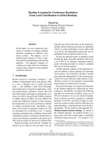
Figure 3: Subgraph of Local
∗
1
output for“headache”
ods are sensitive to parameter tuning and in the
absence of a development set their performance
dramatically deteriorates.
To further establish the merits of global algo-
rithms, we compare (Table 2) tuned-LP, the best
global algorithm, with Local
∗
1
, the best local al-
gorithm. The table considers all edges where the
two algorithms disagree, and counts how many
are in the gold standard and how many are not.
Clearly, tuned-LP is superior at avoiding wrong
edges (false positives). This is because tuned-

LP refrains from adding edges that subsequently
induce many undesirable edges through transitiv-
ity. Figures 2 and 3 illustrate this by compar-
ing tuned-LP and Local
∗
1
on a subgraph of the
Headache concept, before adding missing edges
to satisfy transitivity to Local
∗
1
. Note that Local
∗
1
inserts a single wrong edge X-report-headache →
X-prevent-headache, which leads to adding 8 more
wrong edges. This is the type of global considera-
tion that is addressed in an ILP formulation, but is
ignored in a local approach and often overlooked
when employing a greedy algorithm. Figure 2 also
illustrates the utility of a local entailment graph for
information presentation. Presenting information
according to this subgraph distinguishes between
propositions dealing with headache treatments and
1227
propositions dealing with headache risk groups.
Comparing our use of an ILP algorithm to
the greedy one reveals that tuned-LP significantly
outperforms its greedy counterpart on both mea-
sures (p<.01). However, untuned-LP is practically

equivalent to its greedy counterpart. This indicates
that in this experiment the greedy algorithm pro-
vides a good approximation for the optimal solu-
tion achieved by our LP formulation.
Last, when comparing WordNet to local distri-
butional similarity methods, we observe low recall
and high precision, as expected. However, global
methods achieve much higher recall than WordNet
while maintaining comparable precision.
The results clearly demonstrate that a global ap-
proach improves performance on the entailment
graph learning task, and the overall advantage of
employing an ILP solver rather than a greedy al-
gorithm.
7 Conclusion
This paper presented a global optimization algo-
rithm for learning entailment relations between
predicates represented as propositional templates.
We modeled the problem as a graph learning prob-
lem, and searched for the best graph under a global
transitivity constraint. We used Integer Linear
Programming to solve the optimization problem,
which is theoretically sound, and demonstrated
empirically that this method outperforms local al-
gorithms as well as a greedy optimization algo-
rithm on the graph learning task.
Currently, we are investigating a generalization
of our probabilistic formulation that includes a
prior on the edges, and the relation of this prior
to the regularization term introduced in our score-

based formulation. In future work, we would like
to learn general entailment graphs over a large
number of nodes. This will introduce a challenge
to our current optimization algorithm due to com-
plexity issues, and will require careful handling of
predicate ambiguity. Additionally, we will inves-
tigate novel features for the entailment classifier.
This paper used distributional similarity, but other
sources of information are likely to improve per-
formance further.
Acknowledgments
We would like to thank Roy Bar-Haim, David
Carmel and the anonymous reviewers for their
useful comments. We also thank Dafna Berant
and the nine students who prepared the gold stan-
dard data set. This work was developed under
the collaboration of FBK-irst/University of Haifa
and was partially supported by the Israel Science
Foundation grant 1112/08. The first author is
grateful to the Azrieli Foundation for the award of
an Azrieli Fellowship, and has carried out this re-
search in partial fulllment of the requirements for
the Ph.D. degree.
References
Luisa Bentivogli, Ido Dagan, Hoa Trang Dang, Danilo
Giampiccolo, and Bernarde Magnini. 2009. The
fifth Pascal recognizing textual entailment chal-
lenge. In Proceedings of TAC-09.
Rahul Bhagat, Patrick Pantel, and Eduard Hovy. 2007.
LEDIR: An unsupervised algorithm for learning di-

rectionality of inference rules. In Proceedings of
EMNLP-CoNLL.
Alexander Budanitsky and Graeme Hirst. 2006. Eval-
uating wordnet-based measures of lexical semantic
relatedness. Computational Linguistics, 32(1):13–
47.
James Clarke and Mirella Lapata. 2008. Global in-
ference for sentence compression: An integer linear
programming approach. Journal of Artificial Intelli-
gence Research, 31:273–381.
Michael Connor and Dan Roth. 2007. Context sensi-
tive paraphrasing with a single unsupervised classi-
fier. In Proceedings of ECML.
Ido Dagan, Bill Dolan, Bernardo Magnini, and Dan
Roth. 2009. Recognizing textual entailment: Ratio-
nal, evaluation and approaches. Natural Language
Engineering, 15(4):1–17.
Christiane Fellbaum, editor. 1998. WordNet: An Elec-
tronic Lexical Database (Language, Speech, and
Communication). The MIT Press.
Jenny Rose Finkel and Christopher D. Manning. 2008.
Enforcing transitivity in coreference resolution. In
Proceedings of ACL-08: HLT, Short Papers.
Mark Hall, Eibe Frank, Geoffrey Holmes, Bernhard
Pfahringer, Peter Reutemann, and Ian H. Witten.
2009. The WEKA data mining software: An up-
date. SIGKDD Explorations, 11(1).
Thomas Hofmann. 1999. The cluster-abstraction
model: Unsupervised learning of topic hierarchies
from text data. In Proceedings of IJCAI.

Thorsten Joachims. 2005. A support vector method for
multivariate performance measures. In Proceedings
of ICML.
1228
Mika Kaki. 2005. Findex: Search results categories
help users when document ranking fails. In Pro-
ceedings of CHI.
Dekang Lin and Patrick Pantel. 2001. Discovery of in-
ference rules for question answering. Natural Lan-
guage Engineering, 7(4):343–360.
Dekang Lin. 1998. Dependency-based evaluation of
Minipar. In Proceedings of the Workshop on Evalu-
ation of Parsing Systems at LREC.
Andre Martins, Noah Smith, and Eric Xing. 2009.
Concise integer linear programming formulations
for dependency parsing. In Proceedings of ACL.
Vladimir Nikulin. 2008. Classification of imbalanced
data with random sets and mean-variance filtering.
IJDWM, 4(2):63–78.
Dan Roth and Wen tau Yih. 2005. Integer linear pro-
gramming inference for conditional random fields.
In Proceedings of ICML, pages 737–744.
Satoshi Sekine. 2005. Automatic paraphrase discovery
based on context and keywords between ne pairs. In
Proceedings of IWP.
Sideny Siegel and N. John Castellan. 1988. Non-
parametric Statistics for the Behavioral Sciences.
McGraw-Hill, New-York.
Noah Smith and Jason Eisner. 2005. Contrastive es-
timation: Training log-linear models on unlabeled

data. In Proceedings of ACL.
Rion Snow, Daniel Jurafsky, and Andrew Y. Ng. 2005.
Learning syntactic patterns for automatic hypernym
discovery. In Proceedings of NIPS.
Rion Snow, Daniel Jurafsky, and Andrew Y. Ng. 2006.
Semantic taxonomy induction from heterogenous
evidence. In Proceedings of ACL.
Emilia Stoica, Marti Hearst, and Megan Richardson.
2007. Automating creation of hierarchical faceted
metadata structures. In Proceedings of NAACL-
HLT.
Idan Szpektor and Ido Dagan. 2008. Learning entail-
ment rules for unary templates. In Proceedings of
COLING.
Idan Szpektor and Ido Dagan. 2009. Augmenting
wordnet-based inference with argument mapping.
In Proceedings of TextInfer-2009.
Idan Szpektor, Hristo Tanev, Ido Dagan, and Bonaven-
tura Coppola. 2004. Scaling web-based acquisition
of entailment relations. In Proceedings of EMNLP.
Jason Van Hulse, Taghi Khoshgoftaar, and Amri
Napolitano. 2007. Experimental perspectives on
learning from imbalanced data. In Proceedings of
ICML.
Frank Wilcoxon. 1945. Individual comparisons by
ranking methods. Biometrics Bulletin, 1:80–83.
Alexander Yates and Oren Etzioni. 2009. Unsuper-
vised methods for determining object and relation
synonyms on the web. Journal of Artificial Intelli-
gence Research, 34:255–296.

1229