Báo cáo khoa học: "Domain Adaptation by Constraining Inter-Domain Variability of Latent Feature Representation" docx
Bạn đang xem bản rút gọn của tài liệu. Xem và tải ngay bản đầy đủ của tài liệu tại đây (326.37 KB, 10 trang )
Proceedings of the 49th Annual Meeting of the Association for Computational Linguistics, pages 62–71,
Portland, Oregon, June 19-24, 2011.
c
2011 Association for Computational Linguistics
Domain Adaptation by Constraining Inter-Domain Variability
of Latent Feature Representation
Ivan Titov
Saarland University
Saarbruecken, Germany
Abstract
We consider a semi-supervised setting for do-
main adaptation where only unlabeled data is
available for the target domain. One way to
tackle this problem is to train a generative
model with latent variables on the mixture of
data from the source and target domains. Such
a model would cluster features in both do-
mains and ensure that at least some of the la-
tent variables are predictive of the label on the
source domain. The danger is that these pre-
dictive clusters will consist of features specific
to the source domain only and, consequently,
a classifier relying on such clusters would per-
form badly on the target domain. We in-
troduce a constraint enforcing that marginal
distributions of each cluster (i.e., each latent
variable) do not vary significantly across do-
mains. We show that this constraint is effec-
tive on the sentiment classification task (Pang
et al., 2002), resulting in scores similar to
the ones obtained by the structural correspon-
dence methods (Blitzer et al., 2007) without
the need to engineer auxiliary tasks.
1 Introduction
Supervised learning methods have become a stan-
dard tool in natural language processing, and large
training sets have been annotated for a wide vari-
ety of tasks. However, most learning algorithms op-
erate under assumption that the learning data orig-
inates from the same distribution as the test data,
though in practice this assumption is often violated.
This difference in the data distributions normally re-
sults in a significant drop in accuracy. To address
this problem a number of domain-adaptation meth-
ods has recently been proposed (see e.g., (Daum
´
e
and Marcu, 2006; Blitzer et al., 2006; Bickel et al.,
2007)). In addition to the labeled data from the
source domain, they also exploit small amounts of
labeled data and/or unlabeled data from the target
domain to estimate a more predictive model for the
target domain.
In this paper we focus on a more challenging
and arguably more realistic version of the domain-
adaptation problem where only unlabeled data is
available for the target domain. One of the most
promising research directions on domain adaptation
for this setting is based on the idea of inducing a
shared feature representation (Blitzer et al., 2006),
that is mapping from the initial feature representa-
tion to a new representation such that (1) examples
from both domains ‘look similar’ and (2) an accu-
rate classifier can be trained in this new representa-
tion. Blitzer et al. (2006) use auxiliary tasks based
on unlabeled data for both domains (called pivot fea-
tures) and a dimensionality reduction technique to
induce such shared representation. The success of
their domain-adaptation method (Structural Corre-
spondence Learning, SCL) crucially depends on the
choice of the auxiliary tasks, and defining them can
be a non-trivial engineering problem for many NLP
tasks (Plank, 2009). In this paper, we investigate
methods which do not use auxiliary tasks to induce
a shared feature representation.
We use generative latent variable models (LVMs)
learned on all the available data: unlabeled data for
both domains and on the labeled data for the source
domain. Our LVMs use vectors of latent features
62
to represent examples. The latent variables encode
regularities observed on unlabeled data from both
domains, and they are learned to be predictive of
the labels on the source domain. Such LVMs can
be regarded as composed of two parts: a mapping
from initial (normally, word-based) representation
to a new shared distributed representation, and also
a classifier in this representation. The danger of this
semi-supervised approach in the domain-adaptation
setting is that some of the latent variables will cor-
respond to clusters of features specific only to the
source domain, and consequently, the classifier re-
lying on this latent variable will be badly affected
when tested on the target domain. Intuitively, one
would want the model to induce only those features
which generalize between domains. We encode this
intuition by introducing a term in the learning ob-
jective which regularizes inter-domain difference in
marginal distributions of each latent variable.
Another, though conceptually similar, argument
for our method is coming from theoretical re-
sults which postulate that the drop in accuracy of
an adapted classifier is dependent on the discrep-
ancy distance between the source and target do-
mains (Blitzer et al., 2008; Mansour et al., 2009;
Ben-David et al., 2010). Roughly, the discrepancy
distance is small when linear classifiers cannot dis-
tinguish between examples from different domains.
A necessary condition for this is that the feature ex-
pectations do not vary significantly across domains.
Therefore, our approach can be regarded as mini-
mizing a coarse approximation of the discrepancy
distance.
The introduced term regularizes model expecta-
tions and it can be viewed as a form of a general-
ized expectation (GE) criterion (Mann and McCal-
lum, 2010). Unlike the standard GE criterion, where
a model designer defines the prior for a model ex-
pectation, our criterion postulates that the model ex-
pectations should be similar across domains.
In our experiments, we use a form of Harmonium
Model (Smolensky, 1986) with a single layer of bi-
nary latent variables. Though exact inference with
this class of models is infeasible we use an effi-
cient approximation (Bengio and Delalleau, 2007),
which can be regarded either as a mean-field approx-
imation to the reconstruction error or a determinis-
tic version of the Contrastive Divergence sampling
method (Hinton, 2002). Though such an estimator
is biased, in practice, it yields accurate models. We
explain how the introduced regularizer can be inte-
grated into the stochastic gradient descent learning
algorithm for our model.
We evaluate our approach on adapting sentiment
classifiers on 4 domains: books, DVDs, electronics
and kitchen appliances (Blitzer et al., 2007). The
loss due to transfer to a new domain is very sig-
nificant for this task: in our experiments it was
approaching 9%, in average, for the non-adapted
model. Our regularized model achieves 35% aver-
age relative error reduction with respect to the non-
adapted classifier, whereas the non-regularized ver-
sion demonstrates a considerably smaller reduction
of 26%. Both the achieved error reduction and the
absolute score match the results reported in (Blitzer
et al., 2007) for the best version
1
of the SCL method
(SCL-MI, 36%), suggesting that our approach is a
viable alternative to SCL.
The rest of the paper is structured as follows. In
Section 2 we introduce a model which uses vec-
tors of latent variables to model statistical dependen-
cies between the elementary features. In Section 3
we discuss its applicability in the domain-adaptation
setting, and introduce constraints on inter-domain
variability as a way to address the discovered lim-
itations. Section 4 describes approximate learning
and inference algorithms used in our experiments.
In Section 5 we provide an empirical evaluation of
the proposed method. We conclude in Section 6 with
further examination of the related work.
2 The Latent Variable Model
The adaptation method advocated in this paper is ap-
plicable to any joint probabilistic model which uses
distributed representations, i.e. vectors of latent
variables, to abstract away from hand-crafted fea-
tures. These models, for example, include Restricted
Boltzmann Machines (Smolensky, 1986; Hinton,
2002) and Sigmoid Belief Networks (SBNs) (Saul
et al., 1996) for classification and regression tasks,
Factorial HMMs (Ghahramani and Jordan, 1997)
for sequence labeling problems, Incremental SBNs
for parsing problems (Titov and Henderson, 2007a),
1
Among the versions which do not exploit labeled data from
the target domain.
63
as well as different types of Deep Belief Net-
works (Hinton and Salakhutdinov, 2006). The
power of these methods is in their ability to automat-
ically construct new features from elementary ones
provided by the model designer. This feature induc-
tion capability is especially desirable for problems
where engineering features is a labor-intensive pro-
cess (e.g., multilingual syntactic parsing (Titov and
Henderson, 2007b)), or for multitask learning prob-
lems where the nature of interactions between the
tasks is not fully understood (Collobert and Weston,
2008; Gesmundo et al., 2009).
In this paper we consider classification tasks,
namely prediction of sentiment polarity of a user re-
view (Pang et al., 2002), and model the joint distri-
bution of the binary sentiment label y ∈ {0, 1} and
the multiset of text features x, x
i
∈ X . The hidden
variable vector z (z
i
∈ {0, 1}, i = 1, . . . , m) en-
codes statistical dependencies between components
of x and also dependencies between the label y and
the features x. Intuitively, the model can be regarded
as a logistic regression classifier with latent features.
The model assumes that the features and the latent
variable vector are generated jointly from a globally-
normalized model and then the label y is gener-
ated from a conditional distribution dependent on
z. Both of these distributions, P (x, z) and P (y|z),
are parameterized as log-linear models and, conse-
quently, our model can be seen as a combination of
an undirected Harmonium model (Smolensky, 1986)
and a directed SBN model (Saul et al., 1996). The
formal definition is as follows:
(1) Draw (x, z) ∼ P (x, z|v),
(2) Draw label y ∼ σ(w
0
+
m
i=1
w
i
z
i
),
where v and w are parameters, σ is the logistic sig-
moid function, σ(t) = 1/(1 + e
−t
), and the joint
distribution of (x, z) is given by the Gibbs distribu-
tion:
P (x, z|v) ∝ exp(
|x|
j=1
v
x
j
0
+
n
i=1
v
0i
z
i
+
|x|,n
j,i=1
v
x
j
i
z
i
).
Figure 1 presents the corresponding graphical
model. Note that the arcs between x and z are undi-
rected, whereas arcs between y and z are directed.
The parameters of this model θ = (v, w) can be
estimated by maximizing joint likelihood L(θ) of
labeled data for the source domain {x
(l)
, y
(l)
}
l∈S
L
x
z
y
v
w
Figure 1: The latent variable model: x, z, y are random
variables, dependencies between x and z are parameter-
ized by matrix v, and dependencies between z and y - by
vector w.
and unlabeled data for the source and target domain
{x
(l)
}
l∈S
U
∪T
U
, where S
U
and T
U
stand for the un-
labeled datasets for the source and target domains,
respectively. However, given that, first, amount of
unlabeled data |S
U
∪ T
U
| normally vastly exceeds
the amount of labeled data |S
L
| and, second, the
number of features for each example |x
(l)
| is usually
large, the label y will have only a minor effect on
the mapping from the initial features x to the latent
representation z (i.e. on the parameters v). Conse-
quently, the latent representation induced in this way
is likely to be inappropriate for the classification task
in question. Therefore, we follow (McCallum et al.,
2006) and use a multi-conditional objective, a spe-
cific form of hybrid learning, to emphasize the im-
portance of labels y:
L(θ, α)=α
l∈S
L
log P(y
(l)
|x
(l)
, θ)+
l∈S
U
∪T
U
∪S
L
log P(x
(l)
|θ),
where α is a weight, α > 1.
Direct maximization of the objective is prob-
lematic, as it would require summation over all
the 2
m
latent vectors z. Instead we use a mean-
field approximation. Similarly, an efficient ap-
proximate inference algorithm is used to compute
arg max
y
P (y|x, θ) at testing time. The approxima-
tions are described in Section 4.
3 Constraints on Inter-Domain Variability
As we discussed in the introduction, our goal is
to provide a method for domain adaptation based
on semi-supervised learning of models with dis-
tributed representations. In this section, we first dis-
cuss the shortcomings of domain adaptation with
the above-described semi-supervised approach and
motivate constraints on inter-domain variability of
64
the induced shared representation. Then we pro-
pose a specific form of this constraint based on the
Kullback-Leibler (KL) divergence.
3.1 Motivation for the Constraints
Each latent variable z
i
encodes a cluster or a com-
bination of elementary features x
j
. At least some
of these clusters, when induced by maximizing the
likelihood L(θ, α) with sufficiently large α, will be
useful for the classification task on the source do-
main. However, when the domains are substan-
tially different, these predictive clusters are likely
to be specific only to the source domain. For ex-
ample, consider moving from reviews of electronics
to book reviews: the cluster of features related to
equipment reliability and warranty service will not
generalize to books. The corresponding latent vari-
able will always be inactive on the books domain
(or always active, if negative correlation is induced
during learning). Equivalently, the marginal distri-
bution of this variable will be very different for both
domains. Note that the classifier, defined by the vec-
tor w, is only trained on the labeled source examples
{x
(l)
, y
(l)
}
l∈S
L
and therefore it will rely on such la-
tent variables, even though they do not generalize
to the target domain. Clearly, the accuracy of such
classifier will drop when it is applied to target do-
main examples. To tackle this issue, we introduce a
regularizing term which penalizes differences in the
marginal distributions between the domains.
In fact, we do not need to consider the behavior
of the classifier to understand the rationale behind
the introduction of the regularizer. Intuitively, when
adapting between domains, we are interested in rep-
resentations z which explain domain-independent
regularities rather than in modeling inter-domain
differences. The regularizer favors models which fo-
cus on the former type of phenomena rather than the
latter.
Another motivation for the form of regularization
we propose originates from theoretical analysis of
the domain adaptation problems (Ben-David et al.,
2010; Mansour et al., 2009; Blitzer et al., 2007).
Under the assumption that there exists a domain-
independent scoring function, these analyses show
that the drop in accuracy is upper-bounded by the
quantity called discrepancy distance. The discrep-
ancy distance is dependent on the feature represen-
tation z, and the input distributions for both domains
P
S
(z) and P
T
(z), and is defined as
d
z
(S,T)=max
f,f
|E
P
S
[f(z)=f
(z)]−E
P
T
[f(z)=f
(z)]|,
where f and f
are arbitrary linear classifiers
in the feature representation z. The quantity
E
P
[f(z)=f
(z)] measures the probability mass as-
signed to examples where f and f
disagree. Then
the discrepancy distance is the maximal change in
the size of this disagreement set due to transfer be-
tween the domains. For a more restricted class of
classifiers which rely only on any single feature
2
z
i
, the distance is equal to the maximum over the
change in the distributions P (z
i
). Consequently, for
arbitrary linear classifiers we have:
d
z
(S,T) ≥ max
i=1, ,m
|E
P
S
[z
i
= 1] − E
P
T
[z
i
= 1]|.
It follows that low inter-domain variability of the
marginal distributions of latent variables is a neces-
sary condition for low discrepancy distance. Min-
imizing the difference in the marginal distributions
can be regarded as a coarse approximation to the
minimization of the distance. However, we have
to concede that the above argument is fairly infor-
mal, as the generalization bounds do not directly
apply to our case: (1) our feature representation
is learned from the same data as the classifier, (2)
we cannot guarantee that the existence of a domain-
independent scoring function is preserved under the
learned transformation x→z and (3) in our setting
we have access not only to samples from P (z|x, θ)
but also to the distribution itself.
3.2 The Expectation Criterion
Though the above argument suggests a specific form
of the regularizing term, we believe that the penal-
izer should not be very sensitive to small differ-
ences in the marginal distributions, as useful vari-
ables (clusters) are likely to have somewhat differ-
ent marginal distributions in different domains, but
it should severely penalize extreme differences.
To achieve this goal we instead propose to use the
symmetrized Kullback-Leibler (KL) divergence be-
tween the marginal distributions as the penalty. The
2
We consider only binary features here.
65
derivative of the symmetrized KL divergence is large
when one of the marginal distributions is concen-
trated at 0 or 1 with another distribution still having
high entropy, and therefore such configurations are
severely penalized.
3
Formally, the regularizer G(θ)
is defined as
G(θ) =
m
i=1
D(P
S
(z
i
|θ)||P
T
(z
i
|θ))
+D(P
T
(z
i
|θ)||P
S
(z
i
|θ)), (1)
where P
S
(z
i
) and P
T
(z
i
) stand for the training sam-
ple estimates of the marginal distributions of latent
features, for instance:
P
T
(z
i
= 1|θ) =
1
|T
U
|
l∈T
U
P (z
i
= 1|x
(l)
, θ).
We augment the multi-conditional log-likelihood
L(θ, α) with the weighted regularization term G(θ)
to get the composite objective function:
L
R
(θ, α, β) = L(θ, α) − βG(θ), β > 0.
Note that this regularization term can be regarded
as a form of the generalized expectation (GE) crite-
ria (Mann and McCallum, 2010), where GE criteria
are normally defined as KL divergences between a
prior expectation of some feature and the expecta-
tion of this feature given by the model, where the
prior expectation is provided by the model designer
as a form of weak supervision. In our case, both ex-
pectations are provided by the model but on different
domains.
Note that the proposed regularizer can be trivially
extended to support the multi-domain case (Mansour
et al., 2008) by considering symmetrized KL diver-
gences for every pair of domains or regularizing the
distributions for every domain towards their average.
More powerful regularization terms can also be
motivated by minimization of the discrepancy dis-
tance but their optimization is likely to be expensive,
whereas L
R
(θ, α, β) can be optimized efficiently.
3
An alternative is to use the Jensen-Shannon (JS) diver-
gence, however, our preliminary experiments seem to suggest
that the symmetrized KL divergence is preferable. Though the
two divergences are virtually equivalent when the distributions
are very similar (their ratio tends to a constant as the distribu-
tions go closer), the symmetrized KL divergence stronger penal-
izes extreme differences and this is important for our purposes.
4 Learning and Inference
In this section we describe an approximate learning
algorithm based on the mean-field approximation.
Though we believe that our approach is independent
of the specific learning algorithm, we provide the de-
scription for completeness. We also describe a sim-
ple approximate algorithm for computing P (y|x, θ)
at test time.
The stochastic gradient descent algorithm iter-
ates over examples and updates the weight vector
based on the contribution of every considered exam-
ple to the objective function L
R
(θ, α, β). To com-
pute these updates we need to approximate gradients
of ∇
θ
log P(y
(l)
|x
(l)
, θ) (l ∈ S
L
), ∇
θ
log P(x
(l)
|θ)
(l ∈ S
L
∪ S
U
∪ T
U
) as well as to estimate the con-
tribution of a given example to the gradient of the
regularizer ∇
θ
G(θ). In the next sections we will de-
scribe how each of these terms can be estimated.
4.1 Conditional Likelihood Term
We start by explaining the mean-field approximation
of log P (y|x, θ). First, we compute the means µ =
(µ
1
, . . . , µ
m
):
µ
i
= P (z
i
= 1|x, v) = σ(v
0i
+
|x|
j=1
v
x
j
i
).
Now we can substitute them instead of z to approx-
imate the conditional probability of the label:
P (y = 1|x, θ) =
z
P (y|z, w)P (z|x, v)
∝ σ(w
0
+
m
i=1
w
i
µ
i
).
We use this estimate both at testing time and also
to compute gradients ∇
θ
log P(y
(l)
|x
(l)
, θ) during
learning. The gradients can be computed efficiently
using a form of back-propagation. Note that with
this approximation, we do not need to normalize
over the feature space, which makes the model very
efficient at classification time.
This approximation is equivalent to the computa-
tion of the two-layer perceptron with the soft-max
activation function (Bishop, 1995). However, the
above derivation provides a probabilistic interpreta-
tion of the hidden layer.
4.2 Unlabeled Likelihood Term
In this section, we describe how the unlabeled like-
lihood term is optimized in our stochastic learning
66
algorithm. First, we note that, given the directed
nature of the arcs between z and y, the weights
w do not affect the probability of input x, that is
P (x|θ) = P(x|v).
Instead of directly approximating the gradient
∇
v
log P(x
(l)
|v), we use a deterministic version of
the Contrastive Divergence (CD) algorithm, equiv-
alent to the mean-field approximation of the recon-
struction error used in training autoassociaters (Ben-
gio and Delalleau, 2007). The CD-based estimators
are biased estimators but are guaranteed to converge.
Intuitively, maximizing the likelihood of unlabeled
data is closely related to minimizing the reconstruc-
tion error, that is training a model to discover such
mapping parameters u that z encodes all the neces-
sary information to accurately reproduce x
(l)
from z
for every training example x
(l)
. Formally, the mean-
field approximation to the negated reconstruction er-
ror is defined as
ˆ
L(x
(l)
, v) = log P (x
(l)
|µ, v),
where the means, µ
i
= P(z
i
= 1|x
(l)
, v), are com-
puted as in the preceding section. Note that when
computing the gradient of ∇
v
ˆ
L, we need to take into
account both the forward and backward mappings:
the computation of the means µ from x
(l)
and the
computation of the log-probability of x
(l)
given the
means µ:
d
ˆ
L
dv
ki
=
∂
ˆ
L
∂v
ki
+
∂
ˆ
L
∂µ
i
dµ
i
dv
ki
.
4.3 Regularization Term
The criterion G(θ) is also independent of the classi-
fier parameters w, i.e. G(θ) = G(v), and our goal is
to compute the contribution of a considered example
l to the gradient ∇
v
G(v).
The regularizer G(v) is defined as in equation (1)
and it is a function of the sample-based domain-
specific marginal distributions of latent variables P
S
and P
T
:
P
T
(z
i
= 1|θ) =
1
|T
U
|
l∈T
U
µ
(l)
i
,
where the means µ
(l)
i
= P(z
i
= 1|x
(l)
, v); P
S
can
be re-written analogously. G(v) is dependent on the
parameters v only via the mean activations of the
latent variables µ
(l)
, and contribution of each exam-
ple l can be computed by straightforward differenti-
ation:
dG
(l)
(v)
dv
ki
=(log
p
p
−log
1 − p
1 − p
−
p
p
+
1 − p
1 − p
)
dµ
(l)
i
dv
ki
,
where p = P
S
(z
i
= 1|θ) and p
= P
T
(z
i
= 1|θ)
if l is from the source domain, and, inversely, p =
P
T
(z
i
= 1|θ) and p
= P
S
(z
i
= 1|θ), otherwise.
One problem with the above expression is that
the exact computation of P
S
and P
T
requires re-
computation of the means µ
(l)
for all the exam-
ples after each update of the parameters, resulting
in O(|S
L
∪ S
U
∪ T
U
|
2
) complexity of each iteration
of stochastic gradient descent. Instead, we shuffle
examples and use amortization; we approximate P
S
at update t by:
ˆ
P
(t)
S
(z
i
= 1) =
(1−γ)
ˆ
P
(t−1)
S
(z
i
=1)+γµ
(l)
i
, l∈S
L
∪S
U
ˆ
P
(t−1)
S
(z
i
= 1), otherwise,
where l is an example considered at update t. The
approximation
ˆ
P
T
is computed analogously.
5 Empirical Evaluation
In this section we empirically evaluate our approach
on the sentiment classification task. We start with
the description of the experimental set-up and the
baselines, then we present the results and discuss the
utility of the constraint on inter-domain variability.
5.1 Experimental setting
To evaluate our approach, we consider the same
dataset as the one used to evaluate the SCL
method (Blitzer et al., 2007). The dataset is com-
posed of labeled and unlabeled reviews of four dif-
ferent product types: books, DVDs, electronics and
kitchen appliances. For each domain, the dataset
contains 1,000 labeled positive reviews and 1,000 la-
beled negative reviews, as well as several thousands
of unlabeled examples (4,919 reviews per domain in
average: ranging from 3,685 for DVDs to 5,945 for
kitchen appliances). As in Blitzer et al. (2007), we
randomly split each labelled portion into 1,600 ex-
amples for training and 400 examples for testing.
67
70
75
80
85
Books
70.8
72.7
74.7
76.5
75.6
83.3
DVD Electronics Kitchen Average
Base
NoReg
Reg
Reg+
In-domain
73.3
74.6
74.8
76.2
75.4
82.8
77.6
75.6
73.9
76.6
77.9
78.8
84.6
NoReg+
74.6
76.0
78.9
80.2
85.8
79.0
77.7
83.2
82.1
80.0
86.5
Figure 2: Averages accuracies when transferring to books, DVD, electronics and kitchen appliances domains, and
average accuracy over all 12 domain pairs.
We evaluate the performance of our domain-
adaptation approach on every ordered pair of do-
mains. For every pair, the semi-supervised meth-
ods use labeled data from the source domain and
unlabeled data from both domains. We compare
them with two supervised methods: a supervised
model (Base) which is trained on the source do-
main data only, and another supervised model (In-
domain) which is learned on the labeled data from
the target domain. The Base model can be regarded
as a natural baseline model, whereas the In-domain
model is essentially an upper-bound for any domain-
adaptation method. All the methods, supervised and
semi-supervised, are based on the model described
in Section 2.
Instead of using the full set of bigram and unigram
counts as features (Blitzer et al., 2007), we use a fre-
quency cut-off of 30 to remove infrequent ngrams.
This does not seem to have an adverse effect on the
accuracy but makes learning very efficient: the av-
erage training time for the semi-supervised methods
was about 20 minutes on a standard PC.
We coarsely tuned the parameters of the learning
methods using a form of cross-validation. Both the
parameter of the multi-conditional objective α (see
Section 2) and the weighting for the constraint β (see
Section 3.2) were set to 5. We used 25 iterations of
stochastic gradient descent. The initial learning rate
and the weight decay (the inverse squared variance
of the Gaussian prior) were set to 0.01, and both pa-
rameters were reduced by the factor of 2 every it-
eration the objective function estimate went down.
The size of the latent representation was equal to 10.
The stochastic weight updates were amortized with
the momentum (γ) of 0.99.
We trained the model both without regularization
of the domain variability (NoReg, β = 0), and with
the regularizing term (Reg). For the SCL method
to produce an accurate classifier for the target do-
main it is necessary to train a classifier using both the
induced shared representation and the initial non-
transformed representation. In our case, due to joint
learning and non-convexity of the learning problem,
this approach would be problematic.
4
Instead, we
combine predictions of the semi-supervised mod-
els Reg and NoReg with the baseline out-of-domain
model (Base) using the product-of-experts combina-
tion (Hinton, 2002), the corresponding methods are
called Reg+ and NoReg+, respectively.
In all our models, we augmented the vector z with
an additional component set to 0 for examples in the
source domain and to 1 for the target domain exam-
ples. In this way, we essentially subtracted a un-
igram domain-specific model from our latent vari-
able model in the hope that this will further reduce
the domain dependence of the rest of the model pa-
rameters. In preliminary experiments, this modifica-
tion was beneficial for all the models including the
non-constrained one (NoReg).
5.2 Results and Discussion
The results of all the methods are presented in Fig-
ure 2. The 4 leftmost groups of results correspond
to a single target domain, and therefore each of
4
The latent variables are not likely to learn any useful map-
ping in the presence of observable features. Special training
regimes may be used to attempt to circumvent this problem.
68
them is an average over experiments on 3 domain-
pairs, for instance, the group Books represents an
average over adaptation experiments DVDs→books,
electronics→books, kitchen→books. The rightmost
group of the results corresponds to the average over
all 12 experiments. First, observe that the total drop
in the accuracy when moving to the target domain is
8.9%: from 84.6% demonstrated by the In-domain
classifier to 75.6% shown by the non-adapted Base
classifier. For convenience, we also present the er-
rors due to transfer in a separate Table 1: our best
method (Reg+) achieves 35% relative reduction of
this loss, decreasing the gap to 5.7%.
Now, let us turn to the question of the utility of the
constraints. First, observe that the non-regularized
version of the model (NoReg) often fails to outper-
form the baseline and achieves the scores consider-
ably worse than the results of the regularized ver-
sion (2.6% absolute difference). We believe that
this happens because the clusters induced when opti-
mizing the non-regularized learning objective are of-
ten domain-specific. The regularized model demon-
strates substantially better results slightly beating
the baseline in most cases. Still, to achieve a
larger decrease of the domain-adaptation error, it
was necessary to use the combined models, Reg+
and NoReg+. Here, again, the regularized model
substantially outperforms the non-regularized one
(35% against 26% relative error reduction for Reg+
and NoReg+, respectively).
In Table 1, we also compare the results of
our method with the results of the best ver-
sion of the SCL method (SCL-MI) reported
in Blitzer et al. (2007). The average error reduc-
tions for our method Reg+ and for the SCL method
are virtually equal. However, formally, these two
numbers are not directly comparable. First, the ran-
dom splits are different, though this is unlikely to
result in any significant difference, as the split pro-
portions are the same and the test sets are suffi-
ciently large. Second, the absolute scores achieved
in Blitzer et al. (2007) are slightly worse than those
demonstrated in our experiments both for supervised
and semi-supervised methods. In absolute terms,
our Reg+ method outperforms the SCL method by
more than 1%: 75.6% against 74.5%, in average.
This is probably due to the difference in the used
learning methods: optimization of the Huber loss vs.
D Base NoReg Reg NoReg+ Reg+ SCL-MI
B 10.6 12.4 7.7 8.6 6.7 5.8
D 9.5 8.2 8.0 6.6 7.3 6.1
E 8.2 13.0 9.7 6.8 5.5 5.5
K 7.5 8.8 6.5 4.4 3.3 5.6
Av 8.9 10.6 8.0 6.6 5.7 5.8
Table 1: Drop in the accuracy score due to the transfer
for the 4 domains: (B)ooks, (D)VD, (E)electronics and
(K)itchen appliances, and in average over the domains.
our latent variable model.
5
This comparison sug-
gests that our domain-adaptation method is a viable
alternative to SCL.
Also, it is important to point out that the SCL
method uses auxiliary tasks to induce the shared
feature representation, these tasks are constructed
on the basis of unlabeled data. The auxiliary tasks
and the original problem should be closely related,
namely they should have the same (or similar) set
of predictive features. Defining such tasks can be
a challenging engineering problem. On the senti-
ment classification task in order to construct them
two steps need to be performed: (1) a set of words
correlated with the sentiment label is selected, and,
then (2) prediction of each such word is regarded a
distinct auxiliary problem. For many other domains
(e.g., parsing (Plank, 2009)) the construction of an
effective set of auxiliary tasks is still an open prob-
lem.
6 Related Work
There is a growing body of work on domain adapta-
tion. In this paper, we focus on the class of meth-
ods which induce a shared feature representation.
Another popular class of domain-adaptation tech-
niques assume that the input distributions P(x) for
the source and the target domain share support, that
is every example x which has a non-zero probabil-
ity on the target domain must have also a non-zero
probability on the source domain, and vice-versa.
Such methods tackle domain adaptation by instance
re-weighting (Bickel et al., 2007; Jiang and Zhai,
2007), or, similarly, by feature re-weighting (Sat-
pal and Sarawagi, 2007). In NLP, most features
5
The drop in accuracy for the SCL method in Table 1 is is
computed with respect to the less accurate supervised in-domain
classifier considered in Blitzer et al. (2007), otherwise, the com-
puted drop would be larger.
69
are word-based and lexicons are very different for
different domains, therefore such assumptions are
likely to be overly restrictive.
Various semi-supervised techniques for domain-
adaptation have also been considered, one example
being self-training (McClosky et al., 2006). How-
ever, their behavior in the domain-adaptation set-
ting is not well-understood. Semi-supervised learn-
ing with distributed representations and its applica-
tion to domain adaptation has previously been con-
sidered in (Huang and Yates, 2009), but no attempt
has been made to address problems specific to the
domain-adaptation setting. Similar approaches has
also been considered in the context of topic mod-
els (Xue et al., 2008), however the preference to-
wards induction of domain-independent topics was
not explicitly encoded in the learning objective or
model priors.
A closely related method to ours is that
of (Druck and McCallum, 2010) which performs
semi-supervised learning with posterior regulariza-
tion (Ganchev et al., 2010). Our approach differs
from theirs in many respects. First, they do not fo-
cus on the domain-adaptation setting and do not at-
tempt to define constraints to prevent the model from
learning domain-specific information. Second, their
expectation constraints are estimated from labeled
data, whereas we are trying to match expectations
computed on unlabeled data for two domains.
This approach bears some similarity to the adap-
tation methods standard for the setting where la-
belled data is available for both domains (Chelba
and Acero, 2004; Daum
´
e and Marcu, 2006). How-
ever, instead of ensuring that the classifier param-
eters are similar across domains, we favor models
resulting in similar marginal distributions of latent
variables.
7 Discussion and Conclusions
In this paper we presented a domain-adaptation
method based on semi-supervised learning with dis-
tributed representations coupled with constraints fa-
voring domain-independence of modeled phenom-
ena. Our approach results in competitive domain-
adaptation performance on the sentiment classifica-
tion task, rivalling that of the state-of-the-art SCL
method (Blitzer et al., 2007). Both of these meth-
ods induce a shared feature representation but un-
like SCL our method does not require construction
of any auxiliary tasks in order to induce this repre-
sentation. The primary area of the future work is to
apply our method to structured prediction problems
in NLP, such as syntactic parsing or semantic role la-
beling, where construction of auxiliary tasks proved
problematic. Another direction is to favor domain-
invariability not only of the expectations of individ-
ual variables but rather those of constraint functions
involving latent variables, features and labels.
Acknowledgements
The author acknowledges the support of the Cluster
of Excellence on Multimodal Computing and Inter-
action at Saarland University and thanks the anony-
mous reviewers for their helpful comments and sug-
gestions.
References
Shai Ben-David, John Blitzer, Koby Crammer, Alex
Kulesza, Fernando Pereira, and Jennifer Wortman
Vaughan. 2010. A theory of learning from different
domains. Machine Learning, 79:151–175.
Yoshua Bengio and Olivier Delalleau. 2007. Justify-
ing and generalizing contrastive divergence. Techni-
cal Report TR 1311, Department IRO, University of
Montreal, November.
S. Bickel, M. Br
¨
ueckner, and T. Scheffer. 2007. Dis-
criminative learning for differing training and test dis-
tributions. In Proc. of the International Conference on
Machine Learning (ICML), pages 81–88.
Christopher M. Bishop. 1995. Neural Networks for Pat-
tern Recognition. Oxford University Press, Oxford,
UK.
John Blitzer, Ryan McDonald, and Fernando Pereira.
2006. Domain adaptation with structural correspon-
dence learning. In Proc. of EMNLP.
John Blitzer, Mark Dredze, and Fernando Pereira. 2007.
Biographies, bollywood, boom-boxes and blenders:
Domain adaptation for sentiment classification. In
Proc. 45th Meeting of Association for Computational
Linguistics (ACL), Prague, Czech Republic.
John Blitzer, Koby Crammer, Alex Kulesza, Fernando
Pereira, and Jennifer Wortman. 2008. Learning
bounds for domain adaptation. In Proc. Advances In
Neural Information Processing Systems (NIPS ’07).
Ciprian Chelba and Alex Acero. 2004. Adaptation of
maximum entropy capitalizer: Little data can help a
lot. In Proc. of the Conference on Empirical Meth-
ods for Natural Language Processing (EMNLP), pages
285–292.
70
R. Collobert and J. Weston. 2008. A unified architecture
for natural language processing: Deep neural networks
with multitask learning. In International Conference
on Machine Learning, ICML.
Hal Daum
´
e and Daniel Marcu. 2006. Domain adaptation
for statistical classifiers. Journal of Artificial Intelli-
gence, 26:101–126.
Gregory Druck and Andrew McCallum. 2010. High-
performance semi-supervised learning using discrim-
inatively constrained generative models. In Proc. of
the International Conference on Machine Learning
(ICML), Haifa, Israel.
Kuzman Ganchev, Joao Graca, Jennifer Gillenwater, and
Ben Taskar. 2010. Posterior regularization for struc-
tured latent variable models. Journal of Machine
Learning Research (JMLR), pages 2001–2049.
Andrea Gesmundo, James Henderson, Paola Merlo, and
Ivan Titov. 2009. Latent variable model of syn-
chronous syntactic-semantic parsing for multiple lan-
guages. In CoNLL 2009 Shared Task.
Zoubin Ghahramani and Michael I. Jordan. 1997. Fac-
torial hidden Markov models. Machine Learning,
29:245–273.
G. E. Hinton and R. R. Salakhutdinov. 2006. Reducing
the dimensionality of data with neural networks. Sci-
ence, 313:504–507.
Geoffrey E. Hinton. 2002. Training Products of Experts
by Minimizing Contrastive Divergence. Neural Com-
putation, 14:1771–1800.
Fei Huang and Alexander Yates. 2009. Distributional
representations for handling sparsity in supervised se-
quence labeling. In Proceedings of the Annual Meet-
ing of the Association for Computational Linguistics
(ACL).
Jing Jiang and ChengXiang Zhai. 2007. Instance weight-
ing for domain adaptation in nlp. In Proc. of the
Annual Meeting of the ACL, pages 264–271, Prague,
Czech Republic, June. Association for Computational
Linguistics.
Gideon S. Mann and Andrew McCallum. 2010. General-
ized expectation criteria for semi-supervised learning
with weakly labeled data. Journal of Machine Learn-
ing Research, 11:955–984.
Yishay Mansour, Mehryar Mohri, and Afshin Ros-
tamizadeh. 2008. Domain adaptation with multiple
sources. In Advances in Neural Information Process-
ing Systems.
Yishay Mansour, Mehryar Mohri, and Afshin Ros-
tamizadeh. 2009. Domain adaptation: Learning
bounds and algorithms. In Proceedings of The 22nd
Annual Conference on Learning Theory (COLT 2009),
Montreal, Canada.
Andrew McCallum, Chris Pal, Greg Druck, and Xuerui
Wang. 2006. Multi-conditional learning: Genera-
tive/discriminative training for clustering and classifi-
cation. In AAAI.
David McClosky, Eugene Charniak, and Mark Johnson.
2006. Reranking and self-training for parser adapta-
tion. In Proc. of the Annual Meeting of the ACL and
the International Conference on Computational Lin-
guistics, Sydney, Australia.
B. Pang, L. Lee, and S. Vaithyanathan. 2002. Thumbs
up? Sentiment classification using machine learning
techniques. In Proceedings of the Conference on Em-
pirical Methods in Natural Language Processing.
Barbara Plank. 2009. Structural correspondence learning
for parse disambiguation. In Proceedings of the Stu-
dent Research Workshop at EACL 2009, pages 37–45,
Athens, Greece, April. Association for Computational
Linguistics.
Sandeepkumar Satpal and Sunita Sarawagi. 2007. Do-
main adaptation of conditional probability models via
feature subsetting. In Proceedings of 11th European
Conference on Principles and Practice of Knowledge
Discovery in Databases (PKDD), Warzaw, Poland.
Lawrence K. Saul, Tommi Jaakkola, and Michael I. Jor-
dan. 1996. Mean field theory for sigmoid belief
networks. Journal of Artificial Intelligence Research,
4:61–76.
Paul Smolensky. 1986. Information processing in dy-
namical systems: foundations of harmony theory. In
D. Rumehart and J McCelland, editors, Parallel dis-
tributed processing: explorations in the microstruc-
tures of cognition, volume 1 : Foundations, pages 194–
281. MIT Press.
Ivan Titov and James Henderson. 2007a. Constituent
parsing with Incremental Sigmoid Belief Networks. In
Proc. 45th Meeting of Association for Computational
Linguistics (ACL), pages 632–639, Prague, Czech Re-
public.
Ivan Titov and James Henderson. 2007b. Fast and robust
multilingual dependency parsing with a generative la-
tent variable model. In Proc. of the CoNLL shared
task, Prague, Czech Republic.
G R. Xue, W. Dai, Q. Yang, and Y. Yu. 2008. Topic-
bridged PLSA for cross-domain text classification. In
Proceedings of the SIGIR Conference.
71