Báo cáo khoa học: "Automatic Labelling of Topic Models" doc

Proceedings of the 49th Annual Meeting of the Association for Computational Linguistics, pages 1536–1545,
Portland, Oregon, June 19-24, 2011.
c
2011 Association for Computational Linguistics
Automatic Labelling of Topic Models
Jey Han Lau,
♠♥
Karl Grieser,
♥
David Newman,
♠♦
and Timothy Baldwin
♠♥
♠ NICTA Victoria Research Laboratory
♥ Dept of Computer Science and Software Engineering, University of Melbourne
♦ Dept of Computer Science, University of California Irvine
, , ,
Abstract
We propose a method for automatically la-
belling topics learned via LDA topic models.
We generate our label candidate set from the
top-ranking topic terms, titles of Wikipedia ar-
ticles containing the top-ranking topic terms,
and sub-phrases extracted from the Wikipedia
article titles. We rank the label candidates us-
ing a combination of association measures and
lexical features, optionally fed into a super-
vised ranking model. Our method is shown to
perform strongly over four independent sets of
topics, significantly better than a benchmark
method.

1 Introduction
Topic modelling is an increasingly popular frame-
work for simultaneously soft-clustering terms and
documents into a fixed number of “topics”, which
take the form of a multinomial distribution over
terms in the document collection (Blei et al.,
2003). It has been demonstrated to be highly ef-
fective in a wide range of tasks, including multi-
document summarisation (Haghighi and Vander-
wende, 2009), word sense discrimination (Brody
and Lapata, 2009), sentiment analysis (Titov and
McDonald, 2008), information retrieval (Wei and
Croft, 2006) and image labelling (Feng and Lapata,
2010).
One standard way of interpreting a topic is to use
the marginal probabilities p(w
i
|t
j
) associated with
each term w
i
in a given topic t
j
to extract out the 10
terms with highest marginal probability. This results
in term lists such as:
1
stock market investor fund trading invest-
ment firm exchange companies share

1
Here and throughout the paper, we will represent a topic t
j
via its ranking of top-10 topic terms, based on p(w
i
|t
j
).
which are clearly associated with the domain of
stock market trading. The aim of this research is to
automatically generate topic labels which explicitly
identify the semantics of the topic, i.e. which take us
from a list of terms requiring interpretation to a sin-
gle label, such as STOCK MARKET TRADING in the
above case.
The approach proposed in this paper is to first
generate a topic label candidate set by: (1) sourc-
ing topic label candidates from Wikipedia by query-
ing with the top-N topic terms; (2) identifying the
top-ranked document titles; and (3) further post-
processing the document titles to extract sub-strings.
We translate each topic label into features extracted
from Wikipedia, lexical association with the topic
terms in Wikipedia documents, and also lexical fea-
tures for the component terms. This is used as the
basis of a support vector regression model, which
ranks each topic label candidate.
Our contributions in this work are: (1) the genera-
tion of a novel evaluation framework and dataset for
topic label evaluation; (2) the proposal of a method

for both generating and scoring topic label candi-
dates; and (3) strong in- and cross-domain results
across four independent document collections and
associated topic models, demonstrating the ability
of our method to automatically label topics with re-
markable success.
2 Related Work
Topics are conventionally interpreted via their top-
N terms, ranked based on the marginal probability
p(w
i
|t
j
) in that topic (Blei et al., 2003; Griffiths and
Steyvers, 2004). This entails a significant cognitive
load in interpretation, prone to subjectivity. Topics
are also sometimes presented with manual post-hoc
labelling for ease of interpretation in research pub-
lications (Wang and McCallum, 2006; Mei et al.,
1536
2006). This has obvious disadvantages in terms of
subjectivity, and lack of reproducibility/automation.
The closest work to our method is that of Mei et
al. (2007), who proposed various unsupervised ap-
proaches for automatically labelling topics, based
on: (1) generating label candidates by extracting ei-
ther bigrams or noun chunks from the document col-
lection; and (2) ranking the label candidates based
on KL divergence with a given topic. Their proposed
methodology generates a generic list of label can-

didates for all topics using only the document col-
lection. The best method uses bigrams exclusively,
in the form of the top-1000 bigrams based on the
Student’s t-test. We reimplement their method and
present an empirical comparison in Section 5.3.
In other work, Magatti et al. (2009) proposed a
method for labelling topics induced by a hierarchi-
cal topic model. Their label candidate set is the
Google Directory (gDir) hierarchy, and label selec-
tion takes the form of ontological alignment with
gDir. The experiments presented in the paper are
highly preliminary, although the results certainly
show promise. However, the method is only applica-
ble to a hierarchical topic model and crucially relies
on a pre-existing ontology and the class labels con-
tained therein.
Pantel and Ravichandran (2004) addressed the
more specific task of labelling a semantic class
by applying Hearst-style lexico-semantic patterns
to each member of that class. When presented
with semantically homogeneous, fine-grained near-
synonym clusters, the method appears to work well.
With topic modelling, however, the top-ranking
topic terms tended to be associated and not lexically
similar to one another. It is thus highly questionable
whether their method could be applied to topic mod-
els, but it would certainly be interesting to investi-
gate whether our model could conversely be applied
to the labelling of sets of near-synonyms.
In recent work, Lau et al. (2010) proposed to ap-

proach topic labelling via best term selection, i.e.
selecting one of the top-10 topic terms to label the
overall topic. While it is often possible to label top-
ics with topic terms (as is the case with the stock
market topic above), there are also often cases where
topic terms are not appropriate as labels. We reuse
a selection of the features proposed by Lau et al.
(2010), and return to discuss it in detail in Section 3.
While not directly related to topic labelling,
Chang et al. (2009) were one of the first to propose
human labelling of topic models, in the form of syn-
thetic intruder word and topic detection tasks. In the
intruder word task, they include a term w with low
marginal probability p(w|t) for topic t into the top-
N topic terms, and evaluate how well both humans
and their model are able to detect the intruder.
The potential applications for automatic labelling
of topics are many and varied. In document col-
lection visualisation, e.g., the topic model can be
used as the basis for generating a two-dimensional
representation of the document collection (Newman
et al., 2010a). Regions where documents have a
high marginal probability p(d
i
|t
j
) of being associ-
ated with a given topic can be explicitly labelled
with the learned label, rather than just presented
as an unlabelled region, or presented with a dense

“term cloud” from the original topic. In topic model-
based selectional preference learning (Ritter et al.,
2010;
`
O S
´
eaghdha, 2010), the learned topics can
be translated into semantic class labels (e.g. DAYS
OF THE WEEK), and argument positions for individ-
ual predicates can be annotated with those labels for
greater interpretability/portability. In dynamic topic
models tracking the diachronic evolution of topics
in time-sequenced document collections (Blei and
Lafferty, 2006), labels can greatly enhance the inter-
pretation of what topics are “trending” at any given
point in time.
3 Methodology
The task of automatic labelling of topics is a natural
progression from the best topic term selection task
of Lau et al. (2010). In that work, the authors use
a reranking framework to produce a ranking of the
top-10 topic terms based on how well each term – in
isolation – represents a topic. For example, in our
stock market investor fund trading topic example,
the term trading could be considered as a more rep-
resentative term of the overall semantics of the topic
than the top-ranked topic term stock.
While the best term could be used as a topic la-
bel, topics are commonly ideas or concepts that are
better expressed with multiword terms (for example

STOCK MARKET TRADING), or terms that might not
be in the top-10 topic terms (for example, COLOURS
1537
would be a good label for a topic of the form red
green blue cyan ).
In this paper, we propose a novel method for au-
tomatic topic labelling that first generates topic label
candidates using English Wikipedia, and then ranks
the candidates to select the best topic labels.
3.1 Candidate Generation
Given the size and diversity of English Wikipedia,
we posit that the vast majority of (coherent) topics
or concepts are encapsulated in a Wikipedia article.
By making this assumption, the difficult task of gen-
erating potential topic labels is transposed to find-
ing relevant Wikipedia articles, and using the title of
each article as a topic label candidate.
We first use the top-10 topic terms (based on the
marginal probabilities from the original topic model)
to query Wikipedia, using: (a) Wikipedia’s native
search API; and (b) a site-restricted Google search.
The combined set of top-8 article titles returned
from the two search engines for each topic consti-
tutes the initial set of primary candidates.
Next we chunk parse the primary candidates us-
ing the OpenNLP chunker,
2
and extract out all noun
chunks. For each noun chunk, we generate all com-
ponent n-grams (including the full chunk), out of

which we remove all n-grams which are not in them-
selves article titles in English Wikipedia. For exam-
ple, if the Wikipedia document title were the single
noun chunk United States Constitution, we would
generate the bigrams United States and States Con-
stitution, and prune the latter; we would also gen-
erate the unigrams United, States and Constitution,
all of which exist as Wikipedia articles and are pre-
served.
In this way, an average of 30–40 secondary labels
are produced for each topic based on noun chunk n-
grams. A good portion of these labels are commonly
stopwords or unigrams that are only marginally re-
lated to the topic (an artifact of the n-gram gener-
ation process). To remove these outlier labels, we
use the RACO lexical association method of Grieser
et al. (2011).
RACO (Related Article Conceptual Overlap) uses
Wikipedia’s link structure and category membership
to identify the strength of relationship between arti-
2
/>cles via their category overlap. The set of categories
related to an article is defined as the union of the cat-
egory membership of all outlinks in that article. The
category overlap of two articles (a and b) is the in-
tersection of the related category sets of each article.
The formal definition of this measure is as follows:
|(∪
p∈O(a)
C(p)) ∩ (∪

p∈O(b)
C(p))|
where O(a) is the set of outlinks from article a, and
C(p) is the set of categories of which article p is a
member. This is then normalised using Dice’s co-
efficient to generate a similarity measure. In the in-
stance that a term maps onto multiple Wikipedia ar-
ticles via a disambiguation page, we return the best
RACO score across article pairings for a given term
pair. The final score for each secondary label can-
didate is calculated as the average RACO score with
each of the primary label candidates. All secondary
labels with an average RACO score of 0.1 and above
are added to the label candidate set.
Finally, we add the top-5 topic terms to the set of
candidates, based on the marginals from the origi-
nal topic model. Doing this ensures that there are
always label candidates for all topics (even if the
Wikipedia searches fail), and also allows the pos-
sibility of labeling a topic using its own topic terms,
which was demonstrated by Lau et al. (2010) to be a
baseline source of topic label candidates.
3.2 Candidate Ranking
After obtaining the set of topic label candidates, the
next step is to rank the candidates to find the best la-
bel for each topic. We will first describe the features
that we use to represent label candidates.
3.2.1 Features
A good label should be strongly associated with
the topic terms. To learn the association of a label

candidate with the topic terms, we use several lexical
association measures: pointwise mutual information
(PMI), Student’s t-test, Dice’s coefficient, Pearson’s
χ
2
test, and the log likelihood ratio (Pecina, 2009).
We also include conditional probability and reverse
conditional probability measures, based on the work
of Lau et al. (2010). To calculate the association
measures, we parse the full collection of English
Wikipedia articles using a sliding window of width
1538
20, and obtain term frequencies for the label candi-
dates and topic terms. To measure the association
between a label candidate and a list of topic terms,
we average the scores of the top-10 topic terms.
In addition to the association measures, we in-
clude two lexical properties of the candidate: theraw
number of terms, and the relative number of terms in
the label candidate that are top-10 topic terms.
We also include a search engine score for each
label candidate, which we generate by querying a
local copy of English Wikipedia with the top-10
topic terms, using the Zettair search engine (based
on BM25 term similarity).
3
For a given label candi-
date, we return the average score for the Wikipedia
article(s) associated with it.
3.2.2 Unsupervised and Supervised Ranking

Each of the proposed features can be used as the
basis for an unsupervised model for label candidate
selection, by ranking the label candidates for a given
topic and selecting the top-N. Alternatively, they
can be combined in a supervised model, by training
over topics where we have gold-standard labelling
of the label candidates. For the supervised method,
we use a support vector regression (SVR) model
(Joachims, 2006) over all of the features.
4 Datasets
We conducted topic labelling experiments using
document collections constructed from four distinct
domains/genres, to test the domain/genre indepen-
dence of our method:
BLOGS : 120,000 blog articles dated from August
to October 2008 from the Spinn3r blog dataset
4
BOOKS : 1,000 English language books from the
Internet Archive American Libraries collection
NEWS : 29,000 New York Times news articles
dated from July to September 1999, from the
English Gigaword corpus
PUBMED : 77,000 PubMed biomedical abstracts
published in June 2010
3
/>4
/>The BLOGS dataset contains blog posts that cover
a diverse range of subjects, from product reviews
to casual, conversational messages. The BOOKS
topics, coming from public-domain out-of-copyright

books (with publication dates spanning more than
a century), relate to a wide range of topics includ-
ing furniture, home decoration, religion and art,
and have a more historic feel to them. The NEWS
topics reflect the types and range of subjects one
might expect in news articles such as health, finance,
entertainment, and politics. The PUBMED topics
frequently contain domain-specific terms and are
sharply differentiated from the topics for the other
corpora. We are particularly interested in the perfor-
mance of the method over PUBMED, as it is a highly
specialised domain where we may expect lower cov-
erage of appropriate topic labels within Wikipedia.
We took a standard approach to topic modelling
each of the four document collections: we tokenised,
lemmatised and stopped each document,
5
and cre-
ated a vocabulary of terms that occurred at least
ten times. From this processed data, we created a
bag-of-words representation of each document, and
learned topic models with T = 100 topics in each
case.
To focus our experiments on topics that were rela-
tively more coherent and interpretable, we first used
the method of Newman et al. (2010b) to calculate
the average PMI-score for each topic, and filtered
all topics that had an average PMI-score lower than
0.4. We additionally filtered any topics where less
than 5 of the top-10 topic terms are default nomi-

nal in Wikipedia.
6
The filtering criteria resulted in
45 topics for BLOGS, 38 topics for BOOKS, 60 top-
ics for NEWS, and 85 topics for PUBMED. Man-
ual inspection of the discarded topics indicated that
they were predominantly hard-to-label junk topics or
mixed topics, with limited utility for document/term
clustering.
Applying our label candidate generation method-
ology to these 228 topics produced approximately
6000 labels — an average of 27 labels per topic.
5
OpenNLP is used for tokenization, Morpha for lemmatiza-
tion (Minnen et al., 2001).
6
As determined by POS tagging English Wikipedia with
OpenNLP, and calculating the coarse-grained POS priors (noun,
verb, etc.) for each term.
1539
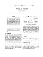
Figure 1: A screenshot of the topic label evaluation task on Amazon Mechanical Turk. This screen constitutes a
Human Intelligence Task (HIT); it contains a topic followed by 10 suggested topic labels, which are to be rated. Note
that been would be the stopword label in this example.
4.1 Topic Candidate Labelling
To evaluate our methods and train the supervised
method, we require gold-standard ratings for the la-
bel candidates. To this end, we used Amazon Me-
chanical Turk to collect annotations for our labels.
In our annotation task, each topic was presented
in the form of its top-10 terms, followed by 10 sug-

gested labels for the topic. This constitutes a Human
Intelligence Task (HIT); annotators are paid based
on the number of HITs they have completed. A
screenshot of a HIT seen by annotator is presented
in Figure 1.
In each HIT, annotators were asked to rate the la-
bels based on the following ordinal scale:
3: Very good label; a perfect description of the
topic.
2: Reasonable label, but does not completely cap-
ture the topic.
1: Label is semantically related to the topic, but
would not make a good topic label.
0: Label is completely inappropriate, and unrelated
to the topic.
To filter annotations from workers who did not
perform the task properly or from spammers, we ap-
1540
Domain Topic Terms Label Candidate
Average
Rating
BLOGS china chinese olympics gold olympic team win beijing medal sport 2008 summer olympics 2.60
BOOKS church arch wall building window gothic nave side vault tower gothic architecture 2.40
NEWS israel peace barak israeli minister palestinian agreement prime leader palestinians israeli-palestinian conflict 2.63
PUBMED cell response immune lymphocyte antigen cytokine t-cell induce receptor immunity immune system 2.36
Table 1: A sample of topics and topic labels, along with the average rating for each label candidate
plied a few heuristics to automatically detect these
workers. Additionally, we inserted a small num-
ber of stopwords as label candidates in each HIT
and recorded workers who gave high ratings to these

stopwords. Annotations from workers who failed to
passed these tests are removed from the final set of
gold ratings.
Each label candidate was rated in this way by at
least 10 annotators, and ratings from annotators who
passed the filter were combined by averaging them.
A sample of topics, label candidates, and the average
rating is presented in Table 1.
7
Finally, we train the regression model over all
the described features, using the human rating-based
ranking.
5 Experiments
In this section we present our experimental results
for the topic labelling task, based on both the unsu-
pervised and supervised methods, and the methodol-
ogy of Mei et al. (2007), which we denote MSZ for
the remainder of the paper.
5.1 Evaluation
We use two basic measures to evaluate the perfor-
mance of our predictions. Top-1 average rating is
the average annotator rating given to the top-ranked
system label, and has a maximum value of 3 (where
annotators unanimously rated all top-ranked system
labels with a 3). This is intended to give a sense of
the absolute utility of the top-ranked candidates.
The second measure is normalized discounted
cumulative gain (nDCG: Jarvelin and Kekalainen
(2002), Croft et al. (2009)), computed for the top-1
(nDCG-1), top-3 (nDCG-3) and top-5 ranked sys-

tem labels (nDCG-5). For a given ordered list of
7
The dataset is available for download from
/>lt/resources/acl2011-topic/.
scores, this measure is based on the difference be-
tween the original order, and the order when the list
is sorted by score. That is, if items are ranked op-
timally in descending order of score at position N,
nDCG-N is equal to 1. nDCG is a normalised score,
and indicates how close the candidate label ranking
is to the optimal ranking within the set of annotated
candidates, noting that an nDCG-N score of 1 tells
us nothing about absolute values of the candidates.
This second evaluation measure is thus intended to
reflect the relative quality of the ranking, and com-
plements the top-1 average rating.
Note that conventional precision- and recall-based
evaluation is not appropriate for our task, as each
label candidate has a real-valued rating.
As a baseline for the task, we use the unsuper-
vised label candidate ranking method based on Pear-
son’s χ
2
test, as it was overwhelmingly found to be
the pick of the features for candidate ranking.
5.2 Results for the Supervised Method
For the supervised model, we present both in-
domain results based on 10-fold cross-validation,
and cross-domain results where we learn a model
from the ratings for the topic model from a given

domain, and apply it to a second domain. In each
case, we learn an SVR model over the full set of fea-
tures described in Section 3.2.1. In practical terms,
in-domain results make the unreasonable assump-
tion that we have labelled 90% of labels in order
to be able to label the remaining 10%, and cross-
domain results are thus the more interesting data
point in terms of the expected results when apply-
ing our method to a novel topic model. It is valuable
to compare the two, however, to gauge the relative
impact of domain on the results.
We present the results for the supervised method
in Table 2, including the unsupervised baseline and
an upper bound estimate for comparison purposes.
The upper bound is calculated by ranking the candi-
1541
Test Domain Training
Top-1 Average Rating
nDCG-1 nDCG-3 nDCG-5
All 1
◦
2
◦
Top5
BLOGS
Baseline (unsupervised) 1.84 1.87 1.75 1.74 0.75 0.77 0.79
In-domain 1.98 1.94 1.95 1.77 0.81 0.82 0.83
Cross-domain: BOOKS 1.88 1.92 1.90 1.77 0.77 0.81 0.83
Cross-domain: NEWS 1.97 1.94 1.92 1.77 0.80 0.83 0.83
Cross-domain: PUBMED 1.95 1.95 1.93 1.82 0.80 0.82 0.83

Upper bound 2.45 2.26 2.29 2.18 1.00 1.00 1.00
BOOKS
Baseline (unsupervised) 1.75 1.76 1.70 1.72 0.77 0.77 0.79
In-domain 1.91 1.90 1.83 1.74 0.84 0.81 0.83
Cross-domain: BLOGS 1.82 1.88 1.79 1.71 0.79 0.81 0.82
Cross-domain: NEWS 1.82 1.87 1.80 1.75 0.79 0.81 0.83
Cross-domain: PUBMED 1.87 1.87 1.80 1.73 0.81 0.82 0.83
Upper bound 2.29 2.17 2.15 2.04 1.00 1.00 1.00
NEWS
Baseline (unsupervised) 1.96 1.76 1.87 1.70 0.80 0.79 0.78
In-domain 2.02 1.92 1.90 1.82 0.82 0.82 0.84
Cross-domain: BLOGS 2.03 1.92 1.89 1.85 0.83 0.82 0.84
Cross-domain: BOOKS 2.01 1.80 1.93 1.73 0.82 0.82 0.83
Cross-domain: PUBMED 2.01 1.93 1.94 1.80 0.82 0.82 0.83
Upper bound 2.45 2.31 2.33 2.12 1.00 1.00 1.00
PUBMED
Baseline (unsupervised) 1.73 1.74 1.68 1.63 0.75 0.77 0.79
In-domain 1.79 1.76 1.74 1.67 0.77 0.82 0.84
Cross-domain: BLOGS 1.80 1.77 1.73 1.69 0.78 0.82 0.84
Cross-domain: BOOKS 1.77 1.70 1.74 1.64 0.77 0.82 0.83
Cross-domain: NEWS 1.79 1.76 1.73 1.65 0.77 0.82 0.84
Upper bound 2.31 2.17 2.22 2.01 1.00 1.00 1.00
Table 2: Supervised results for all domains
dates based on the annotated human ratings. The up-
per bound for top-1 average rating is thus the high-
est average human rating of all label candidates for
a given topic, while the upper bound for the nDCG
measures will always be 1.
In addition to results for the combined candidate
set, we include results for each of the three candi-

date subsets, namely the primary Wikipedia labels
(“1
◦
”), the secondary Wikipedia labels (“2
◦
”) and
the top-5 topic terms (“Top5”); the nDCG results
are over the full candidate set only, as the numbers
aren’t directly comparable over the different subsets
(due to differences in the number of candidates and
the distribution of ratings).
Comparing the in-domain and cross-domain re-
sults, we observe that they are largely compara-
ble, with the exception of BOOKS, where there is
a noticeable drop in both top-1 average rating and
nDGC-1 when we use cross-domain training. We
see an appreciable drop in scores when we train
BOOKS against BLOGS (or vice versa), which we
analyse as being due to incompatibility in document
content and structure between these two domains.
Overall though, the results are very encouraging,
and point to the plausibility of using labelled topic
models from independent domains to learn the best
topic labels for a new domain.
Returning to the question of the suitability of la-
bel candidates for the highly specialised PUBMED
document collection, we first notice that the up-
per bound top-1 average rating is comparable to
the other domains, indicating that our method has
been able to extract equivalent-quality label can-

didates from Wikipedia. The top-1 average rat-
ings of the supervised method are lower than the
other domains. We hypothesise that the cause of
the drop is that the lexical association measures are
trained over highly diverse Wikipedia data rather
than biomedical-specific data, and predict that the
results would improve if we trained our features over
PubMed.
The results are uniformly better than the unsuper-
vised baselines for all four corpora, although there
is quite a bit of room for improvement relative to the
upper bound. To better gauge the quality of these
results, we carry out a direct comparison of our pro-
posed method with the best-performing method of
MSZ in Section 5.3.
1542
Looking to the top-1 average score results over the
different candidate sets, we observe first that the up-
per bound for the combined candidate set (“All”) is
higher than the scores for the candidate subsets in all
cases, underlining the complementarity of the differ-
ent candidate sets. We also observe that the top-5
topic term candidate set is the lowest performer out
of the three subsets across all four corpora, in terms
of both upper bound and the results for the super-
vised method. This reinforces our comments about
the inferiority of the topic word selection method of
Lau et al. (2010) for topic labelling purposes. For
NEWS and PUBMED, there is a noticeable differ-
ence between the results of the supervised method

over the full candidate set and each of the candidate
subsets. In contrast, for BOOKS and BLOGS, the re-
sults for the primary candidate subset are at times
actually higher than those over the full candidate set
in most cases (but not for the upper bound). This is
due to the larger search space in the full candidate
set, and the higher median quality of candidates in
the primary candidate set.
5.3 Comparison with MSZ
The best performing method out of the suite of
approaches proposed by MSZ method exclusively
uses bigrams extracted from the document collec-
tion, ranked based on Student’s t-test. The potential
drawbacks to this approach are: all labels must be
bigrams, there must be explicit token instances of
a given bigram in the document collection for it to
be considered as a label candidate, and furthermore,
there must be enough token instances in the docu-
ment collection for it to have a high t score.
To better understand the performance difference
of our approach to that of MSZ, we perform direct
comparison of our proposed method with the bench-
mark method of MSZ.
5.3.1 Candidate Ranking
First, we compare the candidate ranking method-
ology of our method with that of MSZ, using the
label candidates extracted by the MSZ method.
We first extracted the top-2000 bigrams using the
N-gram Statistics Package (Banerjee and Pedersen,
2003). We then ranked the bigrams for each topic

using the Student’s t-test. We included the top-5 la-
bels generated for each topic by the MSZ method
in our Mechanical Turk annotation task, and use the
annotations to directly compare the two methods.
To measure the performance of candidate rank-
ing between our supervised method and MSZ’s, we
re-rank the top-5 labels extracted by MSZ using
our SVR methodology (in-domain) and compare the
top-1 average rating and nDCG scores. Results are
shown in Table 3. We do not include results for the
BOOKS domain because the text collection is much
larger than the other domains, and the computation
for the MSZ relevance score ranking is intractable
due to the number of n-grams (a significant short-
coming of the method).
Looking at the results for the other domains, it is
clear that our ranking system has the upper hand:
it consistently outperforms MSZ over every evalu-
ation metric.
8
Comparing the top-1 average rating
results back to those in Table 2, we observe that
for all three domains, the results for MSZ are be-
low those of the unsupervised baseline, and well be-
low those of our supervised method. The nDCG re-
sults are more competitive, and the nDCG-3 results
are actually higher than our original results in Ta-
ble 2. It is important to bear in mind, however, that
the numbers are in each case relative to a different la-
bel candidate set. Additionally, the results in Table 3

are based on only 5 candidates, with a relatively flat
gold-standard rating distribution, making it easier to
achieve higher nDCG-5 scores.
5.3.2 Candidate Generation
The method of MSZ makes the implicit assump-
tion that good bigram labels are discoverable within
the document collection. In our method, on the other
hand, we (efficiently) access the much larger and
variable n-gram length set of English Wikipedia ar-
ticle titles, in addition to the top-5 topic terms. To
better understand the differences in label candidate
sets, and the relative coverage of the full label can-
didate set in each case, we conducted another survey
where human users were asked to suggest one topic
label for each topic presented.
The survey consisted, once again, of presenting
annotators with a topic, but in this case, we gave
them the open task of proposing the ideal label for
8
Based on a single ANOVA, the difference in results is sta-
tistically significant at the 5% level for BLOGS, and 1% for
NEWS and PUBMED.
1543
Test Domain
Candidate Ranking Top-1
nDCG-1 nDCG-3 nDCG-5
System Avg. Rating
BLOGS
MSZ 1.26 0.65 0.76 0.87
SVR 1.41 0.75 0.85 0.92

Upper bound 1.87 1.00 1.00 1.00
NEWS
MSZ 1.37 0.73 0.81 0.90
SVR 1.66 0.88 0.90 0.95
Upper bound 1.86 1.00 1.00 1.00
PUBMED
MSZ 1.53 0.77 0.85 0.93
SVR 1.73 0.87 0.91 0.96
Upper bound 1.98 1.00 1.00 1.00
Table 3: Comparison of results for our proposed supervised ranking method (SVR) and that of MSZ
the topic. In this, we did not enforce any restrictions
on the type or size of label (e.g. the number of terms
in the label).
Of the manually-generated gold-standard labels,
approximately 36% were contained in the original
document collection, but 60% were Wikipedia arti-
cle titles. This indicates that our method has greater
potential to generate a label of the quality of the ideal
proposed by a human in a completely open-ended
task.
6 Discussion
On the subject of suitability of using Amazon Me-
chanical Turk for natural language tasks, Snow et al.
(2008) demonstrated that the quality of annotation
is comparable to that of expert annotators. With that
said, the PUBMED topics are still a subject of inter-
est, as these topics often contain biomedical terms
which could be difficult for the general populace to
annotate.
As the number of annotators per topic and the

number of annotations per annotator vary, there is
no immediate way to calculate the inter-annotator
agreement. Instead, we calculated the MAE score
for each candidate, which is an average of the ab-
solute difference between an annotator’s rating and
the average rating of a candidate, summed across all
candidates to get the MAE score for a given corpus.
The MAE scores for each corpus are shown in Ta-
ble 4, noting that a smaller value indicates higher
agreement.
As the table shows, the agreement for the
PUBMED domain is comparable with the other
datasets. BLOGS and NEWS have marginally better
Corpus MAE
BLOGS 0.50
BOOKS 0.56
NEWS 0.52
PUBMED 0.56
Table 4: Average MAE score for label candidate rating
over each corpus
agreement, almost certainly because of the greater
immediacy of the topics, covering everyday areas
such as lifestyle and politics. BOOKS topics are oc-
casionally difficult to label due to the breadth of the
domain; e.g. consider a topic containing terms ex-
tracted from Shakespeare sonnets.
7 Conclusion
This paper has presented the task of topic labelling,
that is the generation and scoring of labels for a
given topic. We generate a set of label candidates

from the top-ranking topic terms, titles of Wikipedia
articles containing the top-ranking topic terms, and
also a filtered set of sub-phrases extracted from the
Wikipedia article titles. We rank the label candidates
using a combination of association measures, lexical
features and an Information Retrieval feature. Our
method is shown to perform strongly over four inde-
pendent sets of topics, and also significantly better
than a competitor system.
Acknowledgements
NICTA is funded by the Australian government as rep-
resented by Department of Broadband, Communication
and Digital Economy, and the Australian Research Coun-
cil through the ICT centre of Excellence programme. DN
has also been supported by a grant from the Institute of
Museum and Library Services, and a Google Research
Award.
1544
References
S. Banerjee and T. Pedersen. 2003. The design, im-
plementation, and use of the Ngram Statistic Package.
In Proceedings of the Fourth International Conference
on Intelligent Text Processing and Computational Lin-
guistics, pages 370–381, Mexico City, February.
D.M. Blei and J.D. Lafferty. 2006. Dynamic topic mod-
els. In ICML 2006.
D.M. Blei, A.Y. Ng, and M.I. Jordan. 2003. Latent
Dirichlet allocation. JMLR, 3:993–1022.
S. Brody and M. Lapata. 2009. Bayesian word sense
induction. In EACL 2009, pages 103–111.

J. Chang, J. Boyd-Graber, S. Gerrish, C. Wang, and
D. Blei. 2009. Reading tea leaves: How humans in-
terpret topic models. In NIPS, pages 288–296.
B. Croft, D. Metzler, and T. Strohman. 2009. Search
Engines: Information Retrieval in Practice. Addison
Wesley.
Y. Feng and M. Lapata. 2010. Topic models for im-
age annotation and text illustration. In Proceedings
of Human Language Technologies: The 11th Annual
Conference of the North American Chapter of the As-
sociation for Computational Linguistics (NAACL HLT
2010), pages 831–839, Los Angeles, USA, June.
K. Grieser, T. Baldwin, F. Bohnert, and L. Sonenberg.
2011. Using ontological and document similarity to
estimate museum exhibit relatedness. ACM Journal
on Computing and Cultural Heritage, 3(3):1–20.
T. Griffiths and M. Steyvers. 2004. Finding scientific
topics. In PNAS, volume 101, pages 5228–5235.
A. Haghighi and L. Vanderwende. 2009. Exploring con-
tent models for multi-document summarization. In
HLT: NAACL 2009, pages 362–370.
K. Jarvelin and J. Kekalainen. 2002. Cumulated gain-
based evaluation of IR techniques. ACM Transactions
on Information Systems, 20(4).
T. Joachims. 2006. Training linear svms in linear time.
In Proceedings of the ACM Conference on Knowledge
Discovery and Data Mining (KDD), pages 217–226,
New York, NY, USA. ACM.
J.H. Lau, D. Newman, S. Karimi, and T. Baldwin. 2010.
Best topic word selection for topic labelling. In Coling

2010: Posters, pages 605–613, Beijing, China.
D. Magatti, S. Calegari, D. Ciucci, and F. Stella. 2009.
Automatic labeling of topics. In ISDA 2009, pages
1227–1232, Pisa, Italy.
Q. Mei, C. Liu, H. Su, and C. Zhai. 2006. A probabilistic
approach to spatiotemporal theme pattern mining on
weblogs. In WWW 2006, pages 533–542.
Q. Mei, X. Shen, and C. Zhai. 2007. Automatic labeling
of multinomial topic models. In SIGKDD, pages 490–
499.
G. Minnen, J. Carroll, and D. Pearce. 2001. Applied
morphological processing of English. Journal of Nat-
ural Language Processing, 7(3):207–223.
D. Newman, T. Baldwin, L. Cavedon, S. Karimi, D. Mar-
tinez, and J. Zobel. 2010a. Visualizing document col-
lections and search results using topic mapping. Jour-
nal of Web Semantics, 8(2-3):169–175.
D. Newman, J.H. Lau, K. Grieser, and T. Baldwin.
2010b. Automatic evaluation of topic coherence. In
Proceedings of Human Language Technologies: The
11th Annual Conference of the North American Chap-
ter of the Association for Computational Linguistics
(NAACL HLT 2010), pages 100–108, Los Angeles,
USA, June. Association for Computational Linguis-
tics.
D.
`
O S
´
eaghdha. 2010. Latent variable models of selec-

tional preference. In ACL 2010.
P. Pantel and D. Ravichandran. 2004. Automatically
labeling semantic classes. In HLT/NAACL-04, pages
321–328.
P. Pecina. 2009. Lexical Association Measures: Collo-
cation Extraction. Ph.D. thesis, Charles University.
A. Ritter, Mausam, and O. Etzioni. 2010. A la-
tent Dirichlet allocation method for selectional pref-
erences. In ACL 2010.
R. Snow, B. O’Connor, D. Jurafsky, and A. Y. Ng. 2008.
Cheap and fast—but is it good?: evaluating non-expert
annotations for natural language tasks. In EMNLP
’08: Proceedings of the Conference on Empirical
Methods in Natural Language Processing, pages 254–
263, Morristown, NJ, USA.
I. Titov and R. McDonald. 2008. Modeling online re-
views with multi-grain topic models. In WWW ’08,
pages 111–120.
X. Wang and A. McCallum. 2006. Topics over time: A
non-Markov continuous-time model of topical trends.
In KDD, pages 424–433.
S. Wei and W.B. Croft. 2006. LDA-based document
models for ad-hoc retrieval. In SIGIR ’06, pages 178–
185.
1545