Báo cáo khoa học: "Learning with Annotation Noise" docx

Proceedings of the 47th Annual Meeting of the ACL and the 4th IJCNLP of the AFNLP, pages 280–287,
Suntec, Singapore, 2-7 August 2009.
c
2009 ACL and AFNLP
Learning with Annotation Noise
Eyal Beigman
Olin Business School
Washington University in St. Louis

Beata Beigman Klebanov
Kellogg School of Management
Northwestern University

Abstract
It is usually assumed that the kind of noise
existing in annotated data is random clas-
sification noise. Yet there is evidence
that differences between annotators are not
always random attention slips but could
result from different biases towards the
classification categories, at least for the
harder-to-decide cases. Under an annota-
tion generation model that takes this into
account, there is a hazard that some of the
training instances are actually hard cases
with unreliable annotations. We show
that these are relatively unproblematic for
an algorithm operating under the 0-1 loss
model, whereas for the commonly used
voted perceptron algorithm, hard training
cases could result in incorrect prediction

on the uncontroversial cases at test time.
1 Introduction
It is assumed, often tacitly, that the kind of
noise existing in human-annotated datasets used in
computational linguistics is random classification
noise (Kearns, 1993; Angluin and Laird, 1988),
resulting from annotator attention slips randomly
distributed across instances. For example, Os-
borne (2002) evaluates noise tolerance of shallow
parsers, with random classification noise taken to
be “crudely approximating annotation errors.” It
has been shown, both theoretically and empiri-
cally, that this type of noise is tolerated well by
the commonly used machine learning algorithms
(Cohen, 1997; Blum et al., 1996; Osborne, 2002;
Reidsma and Carletta, 2008).
Yet this might be overly optimistic. Reidsma
and op den Akker (2008) show that apparent dif-
ferences between annotators are not random slips
of attention but rather result from different biases
annotators might have towards the classification
categories. When training data comes from one
annotator and test data from another, the first an-
notator’s biases are sometimes systematic enough
for a machine learner to pick them up, with detri-
mental results for the algorithm’s performance on
the test data. A small subset of doubly anno-
tated data (for inter-annotator agreement check)
and large chunks of singly annotated data (for
training algorithms) is not uncommon in compu-

tational linguistics datasets; such a setup is prone
to problems if annotators are differently biased.
1
Annotator bias is consistent with a number of
noise models. For example, it could be that an
annotator’s bias is exercised on each and every in-
stance, making his preferred category likelier for
any instance than in another person’s annotations.
Another possibility, recently explored by Beigman
Klebanov and Beigman (2009), is that some items
are really quite clear-cut for an annotator with any
bias, belonging squarely within one particular ca-
tegory. However, some instances – termed hard
cases therein – are harder to decide upon, and this
is where various preferences and biases come into
play. In a metaphor annotation study reported by
Beigman Klebanov et al. (2008), certain markups
received overwhelming annotator support when
people were asked to validate annotations after a
certain time delay. Other instances saw opinions
split; moreover, Beigman Klebanov et al. (2008)
observed cases where people retracted their own
earlier annotations.
To start accounting for such annotator behavior,
Beigman Klebanov and Beigman (2009) proposed
a model where instances are either easy, and then
all annotators agree on them, or hard, and then
each annotator flips his or her own coin to de-
1
The different biases might not amount to much in the

small doubly annotated subset, resulting in acceptable inter-
annotator agreement; yet when enacted throughout a large
number of instances they can be detrimental from a machine
learner’s perspective.
280
cide on a label (each annotator can have a different
“coin” reflecting his or her biases). For annota-
tions generated under such a model, there is a dan-
ger of hard instances posing as easy – an observed
agreement between annotators being a result of all
coins coming up heads by chance. They therefore
define the expected proportion of hard instances in
agreed items as annotation noise. They provide
an example from the literature where an annota-
tion noise rate of about 15% is likely.
The question addressed in this article is: How
problematic is learning from training data with an-
notation noise? Specifically, we are interested in
estimating the degree to which performance on
easy instances at test time can be hurt by the pre-
sence of hard instances in training data.
Definition 1 The hard case bias, τ , is the portion
of easy instances in the test data that are misclas-
sified as a result of hard instances in the training
data.
This article proceeds as follows. First, we show
that a machine learner operating under a 0-1 loss
minimization principle could sustain a hard case
bias of θ(
1

√
N
) in the worst case. Thus, while an-
notation noise is hazardous for small datasets, it is
better tolerated in larger ones. However, 0-1 loss
minimization is computationally intractable for
large datasets (Feldman et al., 2006; Guruswami
and Raghavendra, 2006); substitute loss functions
are often used in practice. While their tolerance to
random classification noise is as good as for 0-1
loss, their tolerance to annotation noise is worse.
For example, the perceptron family of algorithms
handle random classification noise well (Cohen,
1997). We show in section 3.4 that the widely
used Freund and Schapire (1999) voted percep-
tron algorithm could face a constant hard case bias
when confronted with annotation noise in training
data, irrespective of the size of the dataset. Finally,
we discuss the implications of our findings for the
practice of annotation studies and for data utiliza-
tion in machine learning.
2 0-1 Loss
Let a sample be a sequence x
1
, . . . , x
N
drawn uni-
formly from the d-dimensional discrete cube I
d
=

{−1, 1}
d
with corresponding labels y
1
, . . . , y
N
∈
{−1, 1}. Suppose further that the learning al-
gorithm operates by finding a hyperplane (w, ψ),
w ∈ R
d
, ψ ∈ R, that minimizes the empirical er-
ror L(w, ψ) =

j=1 N
[y
j
−sgn(

i=1 d
x
i
j
w
i
−
ψ)]
2
. Let there be H hard cases, such that the an-
notation noise is γ =

H
N
.
2
Theorem 1 In the worst case configuration of in-
stances a hard case bias of τ = θ(
1
√
N
) cannot be
ruled out with constant confidence.
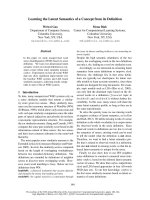
Idea of the proof : We prove by explicit con-
struction of an adversarial case. Suppose there is
a plane that perfectly separates the easy instances.
The θ(N) hard instances will be concentrated in
a band parallel to the separating plane, that is
near enough to the plane so as to trap only about
θ(
√
N) easy instances between the plane and the
band (see figure 1 for an illustration). For a ran-
dom labeling of the hard instances, the central
limit theorem shows there is positive probability
that there would be an imbalance between +1 and
−1 labels in favor of −1s on the scale of
√
N,
which, with appropriate constants, would lead to
the movement of the empirically minimal separa-
tion plane to the right of the hard case band, mis-

classifying the trapped easy cases.
Proof : Let v = v(x) =

i=1 d
x
i
denote the
sum of the coordinates of an instance in I
d
and
take λ
e
=
√
d · F
−1
(
√
γ · 2
−
d
2
+
1
2
) and λ
h
=
√
d · F

−1
(γ +
√
γ · 2
−
d
2
+
1
2
), where F (t) is the
cumulative distribution function of the normal dis-
tribution. Suppose further that instances x
j
such
that λ
e
< v
j
< λ
h
are all and only hard instances;
their labels are coinflips. All other instances are
easy, and labeled y = y(x) = sgn(v). In this case,
the hyperplane
1
√
d
(1 . . . 1) is the true separation
plane for the easy instances, with ψ = 0. Figure 1

shows this configuration.
According to the central limit theorem, for d, N
large, the distribution of v is well approximated by
N(0,
√
d). If N = c
1
· 2
d
, for some 0 < c
1
< 4,
the second application of the central limit the-
orem ensures that, with high probability, about
γN = c
1
γ2
d
items would fall between λ
e
and λ
h
(all hard), and
√
γ · 2
−
d
2
N = c
1


γ2
d
would fall
between 0 and λ
e
(all easy, all labeled +1).
Let Z be the sum of labels of the hard cases,
Z =

i=1 H
y
i
. Applying the central limit the-
orem a third time, for large N, Z will, with a
high probability, be distributed approximately as
2
In Beigman Klebanov and Beigman (2009), annotation
noise is defined as percentage of hard instances in the agreed
annotations; this implies noise measurement on multiply an-
notated material. When there is just one annotator, no dis-
tinction between easy vs hard instances can be made; in this
sense, all hard instances are posing as easy.
281
0
λ
e
λ
h
Figure 1: The adversarial case for 0-1 loss.

Squares correspond to easy instances, circles – to
hard ones. Filled squares and circles are labeled
−1, empty ones are labeled +1.
N(0,
√
γN ). This implies that a value as low as
−2σ cannot be ruled out with high (say 95%) con-
fidence. Thus, an imbalance of up to 2
√
γN , or of
2

c
1
γ2
d
, in favor of −1s is possible.
There are between 0 and λ
h
about 2
√
c
1

γ2
d
more −1 hard instances than +1 hard instances, as
opposed to c
1


γ2
d
easy instances that are all +1.
As long as c
1
< 2
√
c
1
, i.e. c
1
< 4, the empirically
minimal threshold would move to λ
h
, resulting in
a hard case bias of τ =
√
γ
√
c
1
2
d
(1−γ)·c
1
2
d
= θ(
1
√

N
).
To see that this is the worst case scenario, we
note that 0-1 loss sustained on θ(N ) hard cases
is the order of magnitude of the possible imba-
lance between −1 and +1 random labels, which
is θ(
√
N). For hard case loss to outweigh the loss
on the misclassified easy instances, there cannot
be more than θ(
√
N) of the latter
✷
Note that the proof requires that N = θ(2
d
)
namely, that asymptotically the sample includes
a fixed portion of the instances. If the sample is
asymptotically smaller, then λ
e
will have to be ad-
justed such that λ
e
=
√
d · F
−1
(θ(
1

√
N
) +
1
2
).
According to theorem 1, for a 10K dataset with
15% hard case rate, a hard case bias of about 1%
cannot be ruled out with 95% confidence.
Theorem 1 suggests that annotation noise as
defined here is qualitatively different from more
malicious types of noise analyzed in the agnostic
learning framework (Kearns and Li, 1988; Haus-
sler, 1992; Kearns et al., 1994), where an adver-
sary can not only choose the placement of the hard
cases, but also their labels. In worst case, the 0-1
loss model would sustain a constant rate of error
due to malicious noise, whereas annotation noise
is tolerated quite well in large datasets.
3 Voted Perceptron
Freund and Schapire (1999) describe the voted
perceptron. This algorithm and its many vari-
ants are widely used in the computational lin-
guistics community (Collins, 2002a; Collins and
Duffy, 2002; Collins, 2002b; Collins and Roark,
2004; Henderson and Titov, 2005; Viola and
Narasimhan, 2005; Cohen et al., 2004; Carreras
et al., 2005; Shen and Joshi, 2005; Ciaramita and
Johnson, 2003). In this section, we show that the
voted perceptron can be vulnerable to annotation

noise. The algorithm is shown below.
Algorithm 1 Voted Perceptron
Training
Input: a labeled training set (x
1
, y
1
), . . . , (x
N
, y
N
)
Output: a list of perceptrons w
1
, . . . , w
N
Initialize: t ← 0; w
1
← 0; ψ
1
← 0
for t = 1 . . . N do
ˆy
t
← sign(w
t
, x
t
 + ψ
t

)
w
t+1
← w
t
+
y
t
− ˆy
t
2
· x
t
ψ
t+1
← ψ
t
+
y
t
− ˆy
t
2
· w
t
, x
t

end for
Forecasting

Input: a list of perceptrons w
1
, . . . , w
N
an unlabeled instance x
Output: A forecasted label y
ˆy ←
P
N
t=1
sign(w
t
, x
t
 + ψ
t
)
y ← sign(ˆy)
The voted perceptron algorithm is a refinement
of the perceptron algorithm (Rosenblatt, 1962;
Minsky and Papert, 19 69). Perceptron is a dy-
namic algorithm; starting with an initial hyper-
plane w
0
, it passes repeatedly through the labeled
sample. Whenever an instance is misclassified
by w
t
, the hyperplane is modified to adapt to the
instance. The algorithm terminates once it has

passed through the sample without making any
classification mistakes. The algorithm terminates
iff the sample can be separated by a hyperplane,
and in this case the algorithm finds a separating
hyperplane. Novikoff (1962) gives a bound on the
number of iterations the algorithm goes through
before termination, when the sample is separable
by a margin.
282
The perceptron algorithm is vulnerable to noise,
as even a little noise could make the sample in-
separable. In this case the algorithm would cycle
indefinitely never meeting termination conditions,
w
t
would obtain values within a certain dynamic
range but would not converge. In such setting,
imposing a stopping time would be equivalent to
drawing a random vector from the dynamic range.
Freund and Schapire (1999) extend the percep-
tron to inseparable samples with their voted per-
ceptron algorithm and give theoretical generaliza-
tion bounds for its performance. The basic idea
underlying the algorithm is that if the dynamic
range of the perceptron is not too large then w
t
would classify most instances correctly most of
the time (for most values of t). Thus, for a sample
x
1

, . . . , x
N
the new algorithm would keep track
of w
0
, . . . , w
N
, and for an unlabeled instance x it
would forecast the classification most prominent
amongst these hyperplanes.
The bounds given by Freund and Schapire
(1999) depend on the hinge loss of the dataset. In
section 3.2 we construct a difficult setting for this
algorithm. To prove that voted perceptron would
suffer from a constant hard case bias in this set-
ting using the exact dynamics of the perceptron is
beyond the scope of this article. Instead, in sec-
tion 3.3 we provide a lower bound on the hinge
loss for a simplified model of the perceptron algo-
rithm dynamics, which we argue would be a good
approximation to the true dynamics in the setting
we constructed. For this simplified model, we
show that the hinge loss is large, and the bounds
in Freund and Schapire (1999) cannot rule out a
constant level of error regardless of the size of the
dataset. In section 3.4 we study the dynamics of
the model and prove that τ = θ(1) for the adver-
sarial setting.
3.1 Hinge Loss
Definition 2 The hinge loss of a labeled instance

(x, y) with respect to hyperplane (w, ψ) and mar-
gin δ > 0 is given by ζ = ζ(ψ, δ) = max(0, δ −
y · (w, x −ψ)).
ζ measures the distance of an instance from
being classified correctly with a δ margin. Figure 2
shows examples of hinge loss for various data
points.
Theorem 2 (Freund and Schapire (1999))
After one pass on the sample, the probability
that the voted perceptron algorithm does not
δ
ζ
ζ
ζ
ζ
ζ
ζ
Figure 2: Hinge loss ζ for various data points in-
curred by the separator with margin δ.
predict correctly the label of a test instance
x
N+1
is bounded by
2
N+1
E
N+1

d+D
δ


2
where
D = D(w, ψ, δ) =


N
i=1
ζ
2
i
.
This result is used to explain the convergence of
weighted or voted perceptron algorithms (Collins,
2002a). It is useful as long as the expected value of
D is not too large. We show that in an adversarial
setting of the annotation noise D is large, hence
these bounds are trivial.
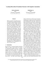
3.2 Adversarial Annotation Noise
Let a sample be a sequence x
1
, . . . , x
N
drawn uni-
formly from I
d
with y
1
, . . . , y
N

∈ {−1, 1}. Easy
cases are labeled y = y(x) = sgn(v) as before,
with v = v(x) =

i=1 d
x
i
. The true separation
plane for the easy instances is w
∗
=
1
√
d
(1 . . . 1),
ψ
∗
= 0. Suppose hard cases are those where
v(x) > c
1
√
d, where c
1
is chosen so that the
hard instances account for γN of all instances.
3
Figure 3 shows this setting.
3.3 Lower Bound on Hinge Loss
In the simplified case, we assume that the algo-
rithm starts training with the hyperplane w

0
=
w
∗
=
1
√
d
(1 . . . 1), and keeps it throughout the
training, only updating ψ. In reality, each hard in-
stance can be decomposed into a component that is
parallel to w
∗
, and a component that is orthogonal
to it. The expected contribution of the orthogonal
3
See the proof of 0-1 case for a similar construction using
the central limit theorem.
283
0 c
1
√d
Figure 3: An adversarial case of annotation noise
for the voted perceptron algorithm.
component to the algorithm’s update will be posi-
tive due to the systematic positioning of the hard
cases, while the contributions of the parallel com-
ponents are expected to cancel out due to the sym-
metry of the hard cases around the main diagonal
that is orthogonal to w

∗
. Thus, while w
t
will not
necessarily parallel w
∗
, it will be close to parallel
for most t > 0. The simplified case is thus a good
approximation of the real case, and the bound we
obtain is expected to hold for the real case as well.
For any initial value ψ
0
< 0 all misclassified in-
stances are labeled −1 and classified as +1, hence
the update will increase ψ
0
, and reach 0 soon
enough. We can therefore assume that ψ
t
≥ 0
for any t > t
0
where t
0
 N .
Lemma 3 For any t > t
0
, there exist α =
α(γ, T) > 0 such that E(ζ
2

) ≥ α · δ.
Proof : For ψ ≥ 0 there are two main sources
of hinge loss: easy +1 instances that are clas-
sified as −1, and hard -1 instances classified as
+1. These correspond to the two components of
the following sum (the inequality is due to disre-
garding the loss incurred by a correct classification
with too wide a margin):
E(ζ
2
) ≥
[ψ]

l=0
1
2
d

d
l

(
ψ
√
d
−
l
√
d
+ δ)

2
+
1
2
d

l=c
1
√
d
1
2
d

d
l

(
l
√
d
−
ψ
√
d
+ δ)
2
Let 0 < T < c
1
be a parameter. For ψ > T

√
d,
misclassified easy instances dominate the loss:
E(ζ
2
) ≥
[ψ]

l=0
1
2
d

d
l

(
ψ
√
d
−
l
√
d
+ δ)
2
≥
[T
√
d]


l=0
1
2
d

d
l

(
T
√
d
√
d
−
l
√
d
+ δ)
2
≥
T
√
d

l=0
1
2
d


d
l

(T −
l
√
d
+ δ)
2
≥
1
√
2π

T
0
(T + δ − t)
2
e
−t
2
/2
dt = H
T
(δ)
The last inequality follows from a normal ap-
proximation of the binomial distribution (see, for
example, Feller (1968)).
For 0 ≤ ψ ≤ T

√
d, misclassified hard cases
dominate:
E(ζ
2
) ≥
1
2
d

l=c
1
√
d
1
2
d

d
l

(
l
√
d
−
ψ
√
d
+ δ)

2
≥
1
2
d

l=c
1
√
d
1
2
d

d
l

(
l
√
d
−
T
√
d
√
d
+ δ)
2
≥

1
2
·
1
√
2π

∞
Φ
−1
(γ)
(t − T + δ)
2
e
−t
2
/2
dt
= H
γ
(δ)
where Φ
−1
(γ) is the inverse of the normal distri-
bution density.
Thus E(ζ
2
) ≥ min{H
T
(δ), H

γ
(δ)}, and
there exists α = α(γ, T ) > 0 such that
min{H
T
(δ), H
γ
(δ)} ≥ α · δ
✷
Corollary 4 The bound in theorem 2 does not
converge to zero for large N.
We recall that Freund and Schapire (1999) bound
is proportional to D
2
=

N
i=1
ζ
2
i
. It follows from
lemma 3 that D
2
= θ(N ), hence the bound is in-
effective.
3.4 Lower Bound on τ for Voted Perceptron
Under Simplified Dynamics
Corollary 4 does not give an estimate on the hard
case bias. Indeed, it could be that w

t
= w
∗
for
almost every t. There would still be significant
hinge in this case, but the hard case bias for the
voted forecast would be zero. To assess the hard
case bias we need a model of perceptron dyna-
mics that would account for the history of hyper-
planes w
0
, . . . , w
N
the perceptron goes through on
284
a sample x
1
, . . . , x
N
. The key simplification in
our model is assuming that w
t
parallels w
∗
for all
t, hence the next hyperplane depends only on the
offset ψ
t
. This is a one dimensional Markov ran-
dom walk governed by the distribution

P(ψ
t+1
−ψ
t
= r|ψ
t
) = P(x|
y
t
− ˆy
t
2
·w
∗
, x = r)
In general −d ≤ ψ
t
≤ d but as mentioned before
lemma 3, we may assume ψ
t
> 0.
Lemma 5 There exists c > 0 such that with a high
probability ψ
t
> c ·
√
d for most 0 ≤ t ≤ N.
Proof : Let c
0
= F

−1
(
γ
2
+
1
2
); c
1
= F
−1
(1−γ).
We designate the intervals I
0
= [0, c
0
·
√
d]; I
1
=
[c
0
·
√
d, c
1
·
√
d] and I

2
= [c
1
·
√
d, d] and define
A
i
= {x : v(x) ∈ I
i
} for i = 0, 1, 2. Note that the
constants c
0
and c
1
are chosen so that P(A
0
) =
γ
2
and P(A
2
) = γ. It follows from the construction
in section 3.2 that A
0
and A
1
are easy instances
and A
2

are hard. Given a sample x
1
, . . . , x
N
, a
misclassification of x
t
∈ A
0
by ψ
t
could only hap-
pen when an easy +1 instance is classified as −1.
Thus the algorithm would shift ψ
t
to the left by
no more than |v
t
− ψ
t
| since v
t
= w
∗
, x
t
. This
shows that ψ
t
∈ I

0
implies ψ
t+1
∈ I
0
. In the
same manner, it is easy to verify that if ψ
t
∈ I
j
and x
t
∈ A
k
then ψ
t+1
∈ I
k
, unless j = 0 and
k = 1, in which case ψ
t+1
∈ I
0
because x
t
∈ A
1
would be classified correctly by ψ
t
∈ I

0
.
We construct a Markov chain with three states
a
0
= 0, a
1
= c
0
·
√
d and a
2
= c
1
·
√
d governed
by the following transition distribution:




1 −
γ
2
0
γ
2
γ

2
1 − γ
γ
2
γ
2
1
2
−
3γ
2
1
2
+ γ




Let X
t
be the state at time t. The principal eigen-
vector of the transition matrix (
1
3
,
1
3
,
1
3

) gives the
stationary probability distribution of X
t
. Thus
X
t
∈ {a
1
, a
2
} with probability
2
3
. Since the tran-
sition distribution of X
t
mirrors that of ψ
t
, and
since a
j
are at the leftmost borders of I
j
, respec-
tively, it follows that X
t
≤ ψ
t
for all t, thus
X

t
∈ {a
1
, a
2
} implies ψ
t
∈ I
1
∪I
2
. It follows that
ψ
t
> c
0
·
√
d with probability
2
3
, and the lemma
follows from the law of large numbers
✷
Corollary 6 With high probability τ = θ(1).
Proof : Lemma 5 shows that for a sample
x
1
, . . . , x
N

with high probability ψ
t
is most of
the time to the right of c ·
√
d. Consequently
for any x in the band 0 ≤ v ≤ c ·
√
d we get
sign(w
∗
, x+ ψ
t
) = −1 for most t hence by defi-
nition, the voted perceptron would classify such
an instance as −1, although it is in fact a +1 easy
instance. Since there are θ(N) misclassified easy
instances, τ = θ(1)
✷
4 Discussion
In this article we show that training with annota-
tion noise can be detrimental for test-time results
on easy, uncontroversial instances; we termed this
phenomenon hard case bias. Although under
the 0-1 loss model annotation noise can be tole-
rated for larger datasets (theorem 1), minimizing
such loss becomes intractable for larger datasets.
Freund and Schapire (1999) voted perceptron al-
gorithm and its variants are widely used in compu-
tational linguistics practice; our results show that

it could suffer a constant rate of hard case bias ir-
respective of the size of the dataset (section 3.4).
How can hard case bias be reduced? One pos-
sibility is removing as many hard cases as one
can not only from the test data, as suggested in
Beigman Klebanov and Beigman (2009), but from
the training data as well. Adding the second an-
notator is expected to detect about half the hard
cases, as they would surface as disagreements be-
tween the annotators. Subsequently, a machine
learner can be told to ignore those cases during
training, reducing the risk of hard case bias. While
this is certainly a daunting task, it is possible that
for annotation studies that do not require expert
annotators and extensive annotator training, the
newly available access to a large pool of inexpen-
sive annotators, such as the Amazon Mechanical
Turk scheme (Snow et al., 2008),
4
or embedding
the task in an online game played by volunteers
(Poesio et al., 2008; von Ahn, 2006) could provide
some solutions.
Reidsma and op den Akker (2008) suggest a
different option. When non-overlapping parts of
the dataset are annotated by different annotators,
each classifier can be trained to reflect the opinion
(albeit biased) of a specific annotator, using dif-
ferent parts of the datasets. Such “subjective ma-
chines” can be applied to a new set of data; an

item that causes disagreement between classifiers
is then extrapolated to be a case of potential dis-
agreement between the humans they replicate, i.e.
4
/>285
a hard case. Our results suggest that, regardless
of the success of such an extrapolation scheme in
detecting hard cases, it could erroneously invali-
date easy cases: Each classifier would presumably
suffer from a certain hard case bias, i.e. classify
incorrectly things that are in fact uncontroversial
for any human annotator. If each such classifier
has a different hard case bias, some inter-classifier
disagreements would occur on easy cases. De-
pending on the distribution of those easy cases in
the feature space, this could invalidate valuable
cases. If the situation depicted in figure 1 corre-
sponds to the pattern learned by one of the clas-
sifiers, it would lead to marking the easy cases
closest to the real separation boundary (those be-
tween 0 and λ
e
) as hard, and hence unsuitable for
learning, eliminating the most informative mate-
rial from the training data.
Reidsma and Carletta (2008) recently showed
by simulation that different types of annotator
behavior have different impact on the outcomes of
machine learning from the annotated data. Our re-
sults provide a theoretical analysis that points in

the same direction: While random classification
noise is tolerable, other types of noise – such as
annotation noise handled here – are more proble-
matic. It is therefore important to develop models
of annotator behavior and of the resulting imper-
fections of the annotated datasets, in order to di-
agnose the potential learning problem and suggest
mitigation strategies.
References
Dana Angluin and Philip Laird. 1988. Learning from
Noisy Examples. Machine Learning, 2(4):343–370.
Beata Beigman Klebanov and Eyal Beigman. 2009.
From Annotator Agreement to Noise Models. Com-
putational Linguistics, accepted for publication.
Beata Beigman Klebanov, Eyal Beigman, and Daniel
Diermeier. 2008. Analyzing Disagreements. In
COLING 2008 Workshop on Human Judgments in
Computational Linguistics, pages 2–7, Manchester,
UK.
Avrim Blum, Alan Frieze, Ravi Kannan, and Santosh
Vempala. 1996. A Polynomial-Time Algorithm for
Learning Noisy Linear Threshold Functions. In Pro-
ceedings of the 37th Annual IEEE Symposium on
Foundations of Computer Science, pages 330–338,
Burlington, Vermont, USA.
Xavier Carreras, Ll
´
uis M
`
arquez, and Jorge Castro.

2005. Filtering-Ranking Perceptron Learning for
Partial Parsing. Machine Learning, 60(1):41–71.
Massimiliano Ciaramita and Mark Johnson. 2003. Su-
persense Tagging of Unknown Nouns in WordNet.
In Proceedings of the Empirical Methods in Natural
Language Processing Conference, pages 168–175,
Sapporo, Japan.
William Cohen, Vitor Carvalho, and Tom Mitchell.
2004. Learning to Classify Email into “Speech
Acts”. In Proceedings of the Empirical Methods
in Natural Language Processing Conference, pages
309–316, Barcelona, Spain.
Edith Cohen. 1997. Learning Noisy Perceptrons by
a Perceptron in Polynomial Time. In Proceedings
of the 38th Annual Symposium on Foundations of
Computer Science, pages 514–523, Miami Beach,
Florida, USA.
Michael Collins and Nigel Duffy. 2002. New Ranking
Algorithms for Parsing and Tagging: Kernels over
Discrete Structures, and the Voted Perceptron. In
Proceedings of the 40th Annual Meeting on Associa-
tion for Computational Linguistics, pages 263–370,
Philadelphia, USA.
Michael Collins and Brian Roark. 2004. Incremen-
tal Parsing with the Perceptron Algorithm. In Pro-
ceedings of the 42nd Annual Meeting on Associa-
tion for Computational Linguistics, pages 111–118,
Barcelona, Spain.
Michael Collins. 2002a. Discriminative Training
Methods for Hidden Markov Hodels: Theory and

Experiments with Perceptron Algorithms. In Pro-
ceedings of the Empirical Methods in Natural Lan-
guage Processing Conference, pages 1–8, Philadel-
phia, USA.
Michael Collins. 2002b. Ranking Algorithms for
Named Entity Extraction: Boosting and the Voted
Perceptron. In Proceedings of the 40th Annual
Meeting on Association for Computational Linguis-
tics, pages 489–496, Philadelphia, USA.
Vitaly Feldman, Parikshit Gopalan, Subhash Khot, and
Ashok Ponnuswami. 2006. New Results for Learn-
ing Noisy Parities and Halfspaces. In Proceedings
of the 47th Annual IEEE Symposium on Foundations
of Computer Science, pages 563–574, Los Alamitos,
CA, USA.
William Feller. 1968. An Introduction to Probability
Theory and Its Application, volume 1. Wiley, New
York, 3rd edition.
Yoav Freund and Robert Schapire. 1999. Large Mar-
gin Classification Using the Perceptron Algorithm.
Machine Learning, 37(3):277–296.
Venkatesan Guruswami and Prasad Raghavendra.
2006. Hardness of Learning Halfspaces with Noise.
In Proceedings of the 47th Annual IEEE Symposium
on Foundations of Computer Science, pages 543–
552, Los Alamitos, CA, USA.
286
David Haussler. 1992. Decision Theoretic General-
izations of the PAC Model for Neural Net and other
Learning Applications. Information and Computa-

tion, 100(1):78–150.
James Henderson and Ivan Titov. 2005. Data-Defined
Kernels for Parse Reranking Derived from Proba-
bilistic Models. In Proceedings of the 43rd Annual
Meeting on Association for Computational Linguis-
tics, pages 181–188, Ann Arbor, Michigan, USA.
Michael Kearns and Ming Li. 1988. Learning in the
Presence of Malicious Errors. In Proceedings of the
20th Annual ACM symposium on Theory of Comput-
ing, pages 267–280, Chicago, USA.
Michael Kearns, Robert Schapire, and Linda Sellie.
1994. Toward Efficient Agnostic Learning. Ma-
chine Learning, 17(2):115–141.
Michael Kearns. 1993. Efficient Noise-Tolerant
Learning from Statistical Queries. In Proceedings
of the 25th Annual ACM Symposium on Theory of
Computing, pages 392–401, San Diego, CA, USA.
Marvin Minsky and Seymour Papert. 1969. Percep-
trons: An Introduction to Computational Geometry.
MIT Press, Cambridge, Mass.
A. B. Novikoff. 1962. On convergence proofs on per-
ceptrons. Symposium on the Mathematical Theory
of Automata, 12:615–622.
Miles Osborne. 2002. Shallow Parsing Using Noisy
and Non-Stationary Training Material. Journal of
Machine Learning Research, 2:695–719.
Massimo Poesio, Udo Kruschwitz, and Chamberlain
Jon. 2008. ANAWIKI: Creating Anaphorically An-
notated Resources through Web Cooperation. In
Proceedings of the 6th International Language Re-

sources and Evaluation Conference, Marrakech,
Morocco.
Dennis Reidsma and Jean Carletta. 2008. Reliability
measurement without limit. Computational Linguis-
tics, 34(3):319–326.
Dennis Reidsma and Rieks op den Akker. 2008. Ex-
ploiting Subjective Annotations. In COLING 2008
Workshop on Human Judgments in Computational
Linguistics, pages 8–16, Manchester, UK.
Frank Rosenblatt. 1962. Principles of Neurodynamics:
Perceptrons and the Theory of Brain Mechanisms.
Spartan Books, Washington, D.C.
Libin Shen and Aravind Joshi. 2005. Incremen-
tal LTAG Parsing. In Proceedings of the Human
Language Technology Conference and Empirical
Methods in Natural Language Processing Confer-
ence, pages 811–818, Vancouver, British Columbia,
Canada.
Rion Snow, Brendan O’Connor, Daniel Jurafsky, and
Andrew Ng. 2008. Cheap and Fast – But is it
Good? Evaluating Non-Expert Annotations for Nat-
ural Language Tasks. In Proceedings of the Empir-
ical Methods in Natural Language Processing Con-
ference, pages 254–263, Honolulu, Hawaii.
Paul Viola and Mukund Narasimhan. 2005. Learning
to Extract Information from Semi-Structured Text
Using a Discriminative Context Free Grammar. In
Proceedings of the 28th Annual International ACM
SIGIR Conference on Research and Development
in Information Retrieval, pages 330–337, Salvador,

Brazil.
Luis von Ahn. 2006. Games with a purpose. Com-
puter, 39(6):92–94.
287