Báo cáo khoa học: "A Note on the Implementation of Hierarchical Dirichlet Processes" docx

Proceedings of the ACL-IJCNLP 2009 Conference Short Papers, pages 337–340,
Suntec, Singapore, 4 August 2009.
c
2009 ACL and AFNLP
A Note on the Implementation of
Hierarchical Dirichlet Processes
Phil Blunsom
∗

Sharon Goldwater
∗

Trevor Cohn
∗

Mark Johnson
†
mark
∗
Department of Informatics
University of Edinburgh
Edinburgh, EH8 9AB, UK
†
Department of Cognitive and Linguistic Sciences
Brown University
Providence, RI, USA
Abstract
The implementation of collapsed Gibbs
samplers for non-parametric Bayesian
models is non-trivial, requiring con-
siderable book-keeping. Goldwater et

al. (2006a) presented an approximation
which significantly reduces the storage
and computation overhead, but we show
here that their formulation was incorrect
and, even after correction, is grossly inac-
curate. We present an alternative formula-
tion which is exact and can be computed
easily. However this approach does not
work for hierarchical models, for which
case we present an efficient data structure
which has a better space complexity than
the naive approach.
1 Introduction
Unsupervised learning of natural language is one
of the most challenging areas in NLP. Recently,
methods from nonparametric Bayesian statistics
have been gaining popularity as a way to approach
unsupervised learning for a variety of tasks,
including language modeling, word and mor-
pheme segmentation, parsing, and machine trans-
lation (Teh et al., 2006; Goldwater et al., 2006a;
Goldwater et al., 2006b; Liang et al., 2007; Finkel
et al., 2007; DeNero et al., 2008). These mod-
els are often based on the Dirichlet process (DP)
(Ferguson, 1973) or hierarchical Dirichlet process
(HDP) (Teh et al., 2006), with Gibbs sampling
as a method of inference. Exact implementation
of such sampling methods requires considerable
bookkeeping of various counts, which motivated
Goldwater et al. (2006a) (henceforth, GGJ06) to

develop an approximation using expected counts.
However, we show here that their approximation
is flawed in two respects: 1) It omits an impor-
tant factor in the expectation, and 2) Even after
correction, the approximation is poor for hierar-
chical models, which are commonly used for NLP
applications. We derive an improved O(1) formula
that gives exact values for the expected counts in
non-hierarchical models. For hierarchical models,
where our formula is not exact, we present an
efficient method for sampling from the HDP (and
related models, such as the hierarchical Pitman-
Yor process) that considerably decreases the mem-
ory footprint of such models as compared to the
naive implementation.
As we have noted, the issues described in this
paper apply to models for various kinds of NLP
tasks; for concreteness, we will focus on n-gram
language modeling for the remainder of the paper,
closely following the presentation in GGJ06.
2 The Chinese Restaurant Process
GGJ06 present two nonparametric Bayesian lan-
guage models: a DP unigram model and an HDP
bigram model. Under the DP model, words in a
corpus w = w
1
. . . w
n
are generated as follows:
G|α

0
, P
0
∼ DP(α
0
, P
0
)
w
i
|G ∼ G
where G is a distribution over an infinite set of
possible words, P
0
(the base distribution of the
DP) determines the probability that an item will
be in the support of G, and α
0
(the concentration
parameter) determines the variance of G.
One way of understanding the predictions that
the DP model makes is through the Chinese restau-
rant process (CRP) (Aldous, 1985). In the CRP,
customers (word tokens w
i
) enter a restaurant with
an infinite number of tables and choose a seat. The
table chosen by the ith customer, z
i
, follows the

distribution:
P (z
i
= k|z
−i
) =

n
z
−i
k
i−1+α
0
, 0 ≤ k < K(z
−i
)
α
0
i−1+α
0
, k = K(z
−i
)
337
The
1
meow
4
cats
2

cats
3
cats
5
a
b
c
d
e f
g
h
Figure 1. A seating assignment describing the state of
a unigram CRP. Letters and numbers uniquely identify
customers and tables. Note that multiple tables may
share a label.
where z
−i
= z
1
. . . z
i−1
are the table assignments
of the previous customers, n
z
−i
k
is the number of
customers at table k in z
−i
, and K(z

−i
) is the total
number of occupied tables. If we further assume
that table k is labeled with a word type 
k
drawn
from P
0
, then the assignment of tokens to tables
defines a distribution over words, with w
i
= 
z
i
.
See Figure 1 for an example seating arrangement.
Using this model, the predictive probability of
w
i
, conditioned on the previous words, can be
found by summing over possible seating assign-
ments for w
i
, and is given by
P (w
i
= w|w
−i
) =
n

w
−i
w
+ α
0
P
0
i − 1 + α
0
(1)
This prediction turns out to be exactly that of the
DP model after integrating out the distribution G.
Note that as long as the base distribution P
0
is
fixed, predictions do not depend on the seating
arrangement z
−i
, only on the count of word w
in the previously observed words (n
w
−i
w
). How-
ever, in many situations, we may wish to estimate
the base distribution itself, creating a hierarchical
model. Since the base distribution generates table
labels, estimates of this distribution are based on
the counts of those labels, i.e., the number of tables
associated with each word type.

An example of such a hierarchical model is the
HDP bigram model of GGJ06, in which each word
type w is associated with its own restaurant, where
customers in that restaurant correspond to words
that follow w in the corpus. All the bigram restau-
rants share a common base distribution P
1
over
unigrams, which must be inferred. Predictions in
this model are as follows:
P
2
(w
i
|h
−i
) =
n
h
−i
(w
i−1
,w
i
)
+ α
1
P
1
(w

i
|h
−i
)
n
h
−i
(w
i−1
,∗)
+ α
1
P
1
(w
i
|h
−i
) =
t
h
−i
w
i
+ α
0
P
0
(w
i

)
t
h
−i
∗
+ α
0
(2)
where h
−i
= (w
−i
, z
−i
), t
h
−i
w
i
is the number of
tables labelled with w
i
, and t
h
−i
∗
is the total num-
ber of occupied tables. Of particular note for our
discussion is that in order to calculate these condi-
tional distributions we must know the table assign-

ments z
−i
for each of the words in w
−i
. Moreover,
in the Gibbs samplers often used for inference in
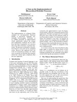
1 10 100 1000
0.1








1








10

100


Mean number of lexical entries
Word frequency (n
w
)


Expectation
Antoniak approx.
Empirical, fixed base
Empirical, inferred base
Figure 2. Comparison of several methods of approx-
imating the number of tables occupied by words of
different frequencies. For each method, results using
α = {100, 1000, 10000, 100000} are shown (from bottom
to top). Solid lines show the expected number of tables,
computed using (3) and assuming P
1
is a fixed uni-
form distribution over a finite vocabulary (values com-
puted using the Digamma formulation (7) are the same).
Dashed lines show the values given by the Antoniak
approximation (4) (the line for α = 100 falls below the
bottom of the graph). Stars show the mean of empirical

table counts as computed over 1000 samples from an
MCMC sampler in which P
1
is a fixed uniform distri-
bution, as in the unigram LM. Circles show the mean
of empirical table counts when P
1
is inferred, as in the
bigram LM. Standard errors in both cases are no larger
than the marker size. All plots are based on the 30114-
word vocabulary and frequencies found in sections 0-20
of the WSJ corpus.
these kinds of models, the counts are constantly
changing over multiple samples, with tables going
in and out of existence frequently. This can create
significant bookkeeping issues in implementation,
and motivated GGJ06 to present a method of com-
puting approximate table counts based on word
frequencies only.
3 Approximating Table Counts
Rather than explicitly tracking the number of
tables t
w
associated with each word w in their
bigram model, GGJ06 approximate the table
counts using the expectation E[t
w
]. Expected
counts are used in place of t
h

−i
w
i
and t
h
−i
∗
in (2).
The exact expectation, due to Antoniak (1974), is
E[t
w
] = α
1
P
1
(w)
n
w

i=1
1
α
1
P
1
(w) + i − 1
(3)
338
Antoniak also gives an approximation to this
expectation:

E[t
w
] ≈ α
1
P
1
(w) log
n
w
+ α
1
P
1
(w)
α
1
P
1
(w)
(4)
but provides no derivation. Due to a misinterpre-
tation of Antoniak (1974), GGJ06 use an approx-
imation that leaves out all the P
1
(w) terms from
(4).
1
Figure 2 compares the approximation to
the exact expectation when the base distribution
is fixed. The approximation is fairly good when

αP
1
(w) > 1 (the scenario assumed by Antoniak);
however, in most NLP applications, αP
1
(w) <
1 in order to effect a sparse prior. (We return
to the case of non-fixed based distributions in a
moment.) As an extreme case of the paucity of
this approximation consider α
1
P
1
(w) = 1 and
n
w
= 1 (i.e. only one customer has entered the
restaurant): clearly E[t
w
] should equal 1, but the
approximation gives log(2).
We now provide a derivation for (4), which will
allow us to obtain an O(1) formula for the expec-
tation in (3). First, we rewrite the summation in (3)
as a difference of fractional harmonic numbers:
2
H
(α
1
P

1
(w)+n
w
−1)
− H
(α
1
P
1
(w)−1)
(5)
Using the recurrence for harmonic numbers:
E[t
w
] ≈ α
1
P
1
(w)

H
(α
1
P
1
(w)+n
w
)
−
1

α
1
P
1
(w) + n
w
− H
(α
1
P
1
(w)+n
w
)
+
1
α
1
P
1
(w)

(6)
We then use the asymptotic expansion,
H
F
≈ log F + γ +
1
2F
, omiting trailing terms

which are O(F
−2
) and smaller powers of F :
3
E[t
w
] ≈ α
1
P
1
(w) log
n
w
+α
1
P
1
(w)
α
1
P
1
(w)
+
n
w
2(α
1
P
1

(w)+n
w
)
Omitting the trailing term leads to the
approximation in Antoniak (1974). However, we
can obtain an exact formula for the expecta-
tion by utilising the relationship between the
Digamma function and the harmonic numbers:
ψ(n) = H
n−1
− γ.
4
Thus we can rewrite (5) as:
5
E[t
w
] = α
1
P
1
(w)·

ψ(α
1
P
1
(w) + n
w
) − ψ(α
1

P
1
(w))

(7)
1
The authors of GGJ06 realized this error, and current
implementations of their models no longer use these approx-
imations, instead tracking table counts explicitly.
2
Fractional harmonic numbers between 0 and 1 are given
by H
F
=
R
1
0
1−x
F
1−x
dx. All harmonic numbers follow the
recurrence H
F
= H
F −1
+
1
F
.
3

Here, γ is the Euler-Mascheroni constant.
4
Accurate O(1) approximations of the Digamma function
are readily available.
5
(7) can be derived from (3) using: ψ(x +1)−ψ(x) =
1
x
.
Explicit table tracking:
customer(w
i
) → table(z
i
)
n
a : 1, b : 1, c : 2, d : 2, e : 3, f : 4, g : 5, h : 5
o
table(z
i
) → label()
n
1 : T he, 2 : cats, 3 : cats, 4 : meow, 5 : cats
o
Histogram:
word type →

table occupancy → frequency

n

T he : {2 : 1}, cats : {1 : 1, 2 : 2}, meow : {1 : 1}
o
Figure 3. The explicit table tracking and histogram rep-
resentations for Figure 1.
A significant caveat here is that the expected
table counts given by (3) and (7) are only valid
when the base distribution is a constant. However,
in hierarchical models such as GGJ06’s bigram
model and HDP models, the base distribution is
not constant and instead must be inferred. As can
be seen in Figure 2, table counts can diverge con-
siderably from the expectations based on fixed
P
1
when P
1
is in fact not fixed. Thus, (7) can
be viewed as an approximation in this case, but
not necessarily an accurate one. Since knowing
the table counts is only necessary for inference
in hierarchical models, but the table counts can-
not be approximated well by any of the formu-
las presented here, we must conclude that the best
inference method is still to keep track of the actual
table counts. The naive method of doing so is to
store which table each customer in the restaurant
is seated at, incrementing and decrementing these
counts as needed during the sampling process. In
the following section, we describe an alternative
method that reduces the amount of memory neces-

sary for implementing HDPs. This method is also
appropriate for hierarchical Pitman-Yor processes,
for which no closed-form approximations to the
table counts have been proposed.
4 Efficient Implementation of HDPs
As we do not have an efficient expected table
count approximation for hierarchical models we
could fall back to explicitly tracking which table
each customer that enters the restaurant sits at.
However, here we describe a more compact repre-
sentation for the state of the restaurant that doesn’t
require explicit table tracking.
6
Instead we main-
tain a histogram for each dish w
i
of the frequency
of a table having a particular number of customers.
Figure 3 depicts the histogram and explicit repre-
sentations for the CRP state in Figure 1.
Our alternative method of inference for hierar-
chical Bayesian models takes advantage of their
6
Teh et al. (2006) also note that the exact table assign-
ments for customers are not required for prediction.
339
Algorithm 1 A new customer enters the restaurant
1: w: word type
2: P
w

0
: Base probability for w
3: HD
w
: Seating Histogram for w
4: procedure INCREMENT(w, P
w
0
, HD
w
)
5: p
share
←
n
w
−1
w
n
w
−1
w
+α
0
 share an existing table
6: p
new
←
α
0

×P
w
0
n
w
−1
w
+α
0
 open a new table
7: r ← random(0, p
share
+ p
new
)
8: if r < p
new
or n
w
−1
w
= 0 then
9: HD
w
[1] = HD
w
[1] + 1
10: else
 Sample from the histogram of customers at tables
11: r ← random(0, n

w
−1
w
)
12: for c ∈ HD
w
do  c: customer count
13: r = r − (c × HD
w
[c])
14: if r ≤ 0 then
15: HD
w
[c] = HD
w
[c] + 1
16: Break
17: n
w
w
= n
w
−1
w
+ 1  Update token count
Algorithm 2 A customer leaves the restaurant
1: w: word type
2: HD
w
: Seating histogram for w

3: procedure DECREMENT(w, P
w
0
, HD
w
)
4: r ← random(0, n
w
w
)
5: for c ∈ HD
w
do  c: customer count
6: r = r − (c × HD
w
[c])
7: if r ≤ 0 then
8: HD
w
[c] = HD
w
[c] − 1
9: if c > 1 then
10: HD
w
[c − 1] = HD
w
[c − 1] + 1
11: Break
12: n

w
w
= n
w
w
− 1  Update token count
exchangeability, which makes it unnecessary to
know exactly which table each customer is seated
at. The only important information is how many
tables exist with different numbers of customers,
and what their labels are. We simply maintain a
histogram for each word type w, which stores, for
each number of customers m, the number of tables
labeled with w that have m customers. Figure 3
depicts the explicit representation and histogram
for the CRP state in Figure 1.
Algorithms 1 and 2 describe the two operations
required to maintain the state of a CRP.
7
When
a customer enters the restaurant (Alogrithm 1)),
we sample whether or not to open a new table.
If not, we sample an old table proportional to the
counts of how many customers are seated there
and update the histogram. When a customer leaves
the restaurant (Algorithm 2), we decrement one
of the tables at random according to the number
of customers seated there. By exchangeability, it
doesn’t actually matter which table the customer
was “really” sitting at.

7
A C++ template class that implements
the algorithm presented is made available at:
/>5 Conclusion
We’ve shown that the HDP approximation pre-
sented in GGJ06 contained errors and inappropri-
ate assumptions such that it significantly diverges
from the true expectations for the most common
scenarios encountered in NLP. As such we empha-
sise that that formulation should not be used.
Although (7) allows E[t
w
] to be calculated exactly
for constant base distributions, for hierarchical
models this is not valid and no accurate calculation
of the expectations has been proposed. As a rem-
edy we’ve presented an algorithm that efficiently
implements the true HDP without the need for
explicitly tracking customer to table assignments,
while remaining simple to implement.
Acknowledgements
The authors would like to thank Tom Grif-
fiths for providing the code used to produce
Figure 2 and acknowledge the support of the
EPSRC (Blunsom, grant EP/D074959/1; Cohn,
grant GR/T04557/01).
References
D. Aldous. 1985. Exchangeability and related topics. In
´
Ecole d’

´
Et
´
e de Probabiliti
´
es de Saint-Flour XIII 1983, 1–
198. Springer.
C. E. Antoniak. 1974. Mixtures of dirichlet processes with
applications to bayesian nonparametric problems. The
Annals of Statistics, 2(6):1152–1174.
J. DeNero, A. Bouchard-C
ˆ
ot
´
e, D. Klein. 2008. Sampling
alignment structure under a Bayesian translation model.
In Proceedings of the 2008 Conference on Empirical
Methods in Natural Language Processing, 314–323, Hon-
olulu, Hawaii. Association for Computational Linguistics.
S. Ferguson. 1973. A Bayesian analysis of some nonpara-
metric problems. Annals of Statistics, 1:209–230.
J. R. Finkel, T. Grenager, C. D. Manning. 2007. The infinite
tree. In Proc. of the 45th Annual Meeting of the ACL
(ACL-2007), Prague, Czech Republic.
S. Goldwater, T. Griffiths, M. Johnson. 2006a. Contex-
tual dependencies in unsupervised word segmentation. In
Proc. of the 44th Annual Meeting of the ACL and 21st
International Conference on Computational Linguistics
(COLING/ACL-2006), Sydney.
S. Goldwater, T. Griffiths, M. Johnson. 2006b. Interpolating

between types and tokens by estimating power-law gener-
ators. In Y. Weiss, B. Sch
¨
olkopf, J. Platt, eds., Advances
in Neural Information Processing Systems 18, 459–466.
MIT Press, Cambridge, MA.
P. Liang, S. Petrov, M. Jordan, D. Klein. 2007. The infinite
PCFG using hierarchical Dirichlet processes. In Proc. of
the 2007 Conference on Empirical Methods in Natural
Language Processing (EMNLP-2007), 688–697, Prague,
Czech Republic.
Y. W. Teh, M. I. Jordan, M. J. Beal, D. M. Blei. 2006.
Hierarchical Dirichlet processes. Journal of the American
Statistical Association, 101(476):1566–1581.
340