The Economic Returns to an MBA∗ pdf
Bạn đang xem bản rút gọn của tài liệu. Xem và tải ngay bản đầy đủ của tài liệu tại đây (236.11 KB, 38 trang )
The Economic Returns to an MBA
∗
Peter Arcidiacono
†
, Jane Cooley
‡
, Andrew Hussey
§
January 3, 2007
Abstract
Estimating the returns to education is difficult in part because we rarely observe the coun-
terfactual of the wages without the education. One of the advantages of examining the returns
to an MBA is that most programs require work experience before being admitted. These obser-
vations on wages allow us to see how productive people are before they actually receive an MBA
and to identify and correct for potential bias in the estimated treatment effect. Controlling for
individual fixed effects generally reduces the estimated returns to an MBA, and especially so for
those in top programs. However, for full-time MBA students attending schools outside of the
top-25 the estimated returns are higher when we control for individual fixed effects. We show
that this arises neither because of a dip in wages before enrolling nor because these individuals
are weaker in observed ability measures than those who do not obtain an MBA. Rather, there
is some evidence that those who take the GMAT but do not obtain an MBA are stronger in
dimensions such as workplace skills that are not easily measured. Including proxies for these
skills substantially reduces the gap between the OLS and fixed effects estimates.
Keywords: Returns to education, ability bias, panel data
JEL: J3, I2, C23
∗
We thank Brad Heim, Paul Ellickson, Bill Johnson, Margie McElroy, Bob Miller, David Ridley, Alessandro Tarozzi,
and participants at the Duke Applied Micro economics Lunch for valuable comments. Suggestions by the editor and
three referees substantially improved the paper. We are grateful to Mark Montgomery for generously providing the
data.
†
Duke University, Department of Economics,
‡
University of Wisconsin-Madison, Department of Economics,
§
University of Memphis, Department of Economics,
1
1 Introduction
While it is generally accepted that more education leads to an increase in wages, an extensive liter-
ature attempts to quantify this effect. The difficulty lies in disentangling the effect of education on
wages from the unobservable personal traits that are correlated with schooling. Because schooling is
usually completed before entrance into the labor market, previous research has relied on instrumen-
tal variables, such as proximity to colleges or date of birth,
1
or exclusion restrictions in a structural
model to identify the effec t of schooling on wages.
2
Alternatively, several studies have used data
on siblings or twins to identify the treatment of additional years of schooling, while controlling for
some degree of innate ability and family environment.
3
We use data on registrants for the Graduate Management Admissions Test (GMAT) – individuals
who were considering obtaining an MBA – to estimate the returns to an MBA and show how these
returns depend upon the method used to control for selection. Unlike most other schooling, MBA
programs generally require work experience . Figure 1 plots the cumulative distribution function for
post-collegiate work experience before enrolling. As shown in the figure, almost ninety percent of
those who enroll in an MBA program have over two years of work experience. That individuals
work before obtaining an MBA allows us to use panel data techniques both to estimate the returns
to an MBA and to quantify the biases associated with not having good controls for ability. The
treatment effect of an MBA on wages is thus identified from wages on the same individual before
and after receiving an MBA.
When the return to an MBA is restricted to be the same across program types and qualities
we estimate a return for males of 9.4%.
4
This coefficient falls by about a third when standard
human capital measures (test scores, grades) are included, and falls by another third to 4.8% when
we control for individual fixed effects, a result consistent with the commonly expected positive
correlation between ability and returns to schooling. This positive ability bias is also reported by
many of the studies using identical twins. However, comparisons across these studies is difficult as
the samples are different and because there may be more measurement error present in retrospective
1
See Angrist and Krueger (1991) and Kane and Rouse (1995) among many others.
2
See Willis and Rosen (1979) and Keane and Wolpin (1997, 2000, 2001).
3
See, for example, Berhman and Taubman (1989), Berhman et al. (1994), Ashenfelter and Krueger (1994) and
Ashenfelter and Rouse (1998).
4
Similar results are seen for females and are reported in section 4.
2
recall of years of schooling than in whether or not one has received an MBA. Furthermore, MBA
programs are geared more directly toward increasing wages or other career-related goals than other
types of schooling which may have broader aims.
5
While disentangling the returns to schooling from the returns to unobserved ability is difficult,
estimating the returns to college quality is harder still. No good instruments have been found
for college quality, and the sample sizes of twins are often too small to obtain accurate estimates
of the returns to college quality.
6
A notable exception is Berhman et al. (1996), who find that,
after controlling for family background characteristics using twins, there are significant returns to
attending colleges of higher “quality” in several observable dimensions. By using data on pre-
MBA wages, we are able to distinguish how the average effect on wages varies across the quality of
programs.
7
Controlling for selection via observables lowers the return to attending a top-10 program
over a program in the lowest tier from 33% to 25%. When fixed effects are included, the gap falls
to 11%. This decline is due to both a drop in the returns to attending a top-10 program, and to an
increase in the return to attending a program outside the top-25. In fact, the somewhat surprising
result is that our OLS estimates show virtually no return for those attending programs outside the
top-25, while the fixed effects estimate s are around eight percent.
Instrumental variable techniques have also found higher returns to schooling than OLS esti-
mates. However, many of the standard reasons given for the higher IV estimates do not hold here.
As discussed in Card (1999, 2001), one explanation for higher IV estimates is that they mitigate
the measurement error problem associated with misreported years of schooling. An alternative ex-
planation applies to the likely case w here the returns to schooling differ across individuals. Then,
IV estimates some weighted average of the heterogeneous treatment effects, which is not directly
5
It is also worth noting that in general the return to schooling literature focuses on the return to an additional year
of schooling, while we measure the return to an MBA as the return to obtaining the degree which is typically 2 years
of schooling. Note that this is a gross return rather than an actual return, and so neglects costs of schooling, taxes,
etc. (see Heckman et al. (2006)).
6
Researchers have attempted to estimate the return to college quality by controlling for selection with observables
(Black et al., 2005; James et al., 1989; Loury and Garman, 1995), matching base d upon similar application and
acceptance sets (Dale and Krueger, 2002; Black and Smith, 2004), and structurally estimating the decision to attend
particular colleges (Brewer et al. (1999), and Arcidiacono (2004, 2005).
7
Programs may differ both in their treatment effects and in costs. Higher costs of top programs may in part explain
their higher average effects, since individuals will only participate in a program if its benefits exceed its costs. Costs
and projected benefits are considered more explicitly in Section 6.
3
comparable to the average treatment effect estimate d by OLS.
8
If the instrument affects a small
subset of the sample with a higher marginal return to schooling, IV estimates will be biased upward
relative to OLS estimates for the same sample. While both of these are potential reasons for the
finding of higher IV estimates, neither applies to fixed effects. In contrast to IV estimates, using
fixed effects tends to exacerbate measurement error, thus biasing estimates toward zero.
9
Further,
both the OLS and fixed effect estimates are of the treatment effect on the treated for a particular
type of program.
Why are the fixed effects estimates higher for those who do not atte nd top-25 schools? While
having wage observations both before and after schooling presents many advantages, it also in-
troduces problems associated with the program evaluation literature.
10
In particular, As henfelter
(1978) documented the dip in earnings which took place before individuals enrolled in job training
programs, something which may also occur when individuals go back to school.
11
Such a dip would
cause us to over-estimate the return to an MBA in a fixed effects framework. However, a similar
dip in wages is not found in our data. We also test for the possibility that individuals with higher
returns to experience are selecting into business school and thus biasing our estimates of the returns
to an MBA upwards.
12
An alternative explanation is that additional schooling could compensate for low workplace skills.
While those who attend full-time MBA programs outside of the top-25 have higher test scores and
higher grades than those who take the GMAT but do not attend, they may be weaker on other
traits which are not easily observable but also important for labor market success. For example,
obtaining an MBA may provide one with job contacts—something those who do not choose to
obtain an MBA may already have. In fact, we are able to show that those who do not obtain an
MBA are actually stronger in areas not generally measured by standard survey data. Controlling
for these factors explains much of the difference be tween the fixed effects and OLS estimates, thus
providing evidence of negative selection into business school conditional on taking the GMAT and
not attending a top-25 program.
8
Heckman and Vytlacil (2005) develop a unifying framework that clarifies the links between the parameters being
estimated using these alternative estimators in the context of he terogeneous treatment effects.
9
See Hsiao (1986) for a discussion of measurement error in panel data models. See also Bertrand et al. (2004).
10
See Heckman et al. (1999) for a review.
11
See Heckman and Smith (1999) for a more recent discussion of the Ashenfelter dip and its effects on longitudinal
estimators of program impact.
12
See Baker (1997). Furthermore, our results are robust to restricting the sample only to those who obtain MBAs.
4
0 1 2 3 4 5 6 7 8 9 10 11 12 13 14 15 16 17 18 19 20
0
0.1
0.2
0.3
0.4
0.5
0.6
0.7
0.8
0.9
1
Figure 1:Empirical CDF of Years of Work Experience Before Enrolling in an MBA Program
Years of Work Experience At Time of Enrollment
Empirical CDF
The one study that uses fixed effects to estimate the returns to schooling – Angrist and Newey
(1991) – finds that fixed effects estimates of the returns to schooling are higher than the correspond-
ing OLS estimates. They suggest that individuals may make up for low workplace productivity by
obtaining more schooling. However, the fixed effects coefficient is identified off of only those who
have a break in schooling, a group which is less than twenty percent of the sample. This is in
contrast to our sample where virtually everyone who obtains an MBA in the sample first obtains
work experience.
While there is a broad literature on the returns to schooling, few studies have investigated
the returns to an MBA. The value of an MBA degree is a concern to potential MBA students,
and articles in the popular press and schools themselves often report average starting salaries of
graduates as an indicator of program effectiveness without addressing issues of selection. The more
rigorous attempts to determine the efficiency or value-added of MBA programs rely on aggregate
data of student characteristics as reported by top-rated schools (Tracy and Waldfogel, 1997; Colbert
et al., 2000; Ray and Jeon, 2003). The purpose of these studies is to rank MBA programs based on
5
their effectiveness after controlling for different observable measures of student quality. They rely
primarily on post-MBA salary information to assess the quality of an MBA program and therefore
cannot control for differences individual fixed effects. An important contribution of our paper,
therefore, is applying individual-level data on student characteristics and pre- and post-MBA wages
to estimate the returns to an MBA, which allows for a more careful treatme nt of s ele ction first into
attending business school and second into programs of varying types and qualities. Other studies
that benefit from data on individual outcomes from attending business school have focused on a
substantively different question, explaining the gender wage gap, rather than estimating the return
to an MBA for various types of MBA programs.
13
The rest of the pap e r proceeds as follows. Section 2 describes the data. A simple model of MBA
attainment and the identification strategy are discussed in Section 3. Estimates of the treatment
effects are presented in Section 4. Section 5 examines possible explanations for the higher fixed
effect estimates for those who attended institutions outside the top-25. In Section 6 we consider
the net benefit of an MBA, after taking into account the varying costs of different types of MBA
programs. Section 7 concludes.
2 Data
We utilize a longitudinal survey of registrants for the Graduate Management Admissions Test
(GMAT) to estimate the ec onomic returns to an MBA. The GMAT exam, an admissions requirement
for most MBA programs, is similar to the SAT for undergraduates without the competition from
the ACT. The survey, sponsored by the Graduate Management Admissions Council (GMAC), was
administered in four waves, beginning in 1990 and ending in 1998.
14
In addition, survey responses
were linked to GMAC’s registration and test data, which includes personal background information
and GMAT scores. The initial sample size surveyed in wave 1 was 7006, of which 5602 actually took
the test. We focus our analysis on the sample of test takers.
The key feature of the data is that we observe wages both before and after an individual receives
an MBA. In Table 1 we show the distribution of the individuals across five activities and the four
13
Graddy and Pistaferri (2000) analyze the extent of the gender wage gap comparing the starting salaries of graduates
of London Business School. Montgomery and Powell (2003) look at changes in the gender wage gap due to MBA
completion, using the same data as in the current study.
14
The same survey has been used by Montgomery (2002) and Montgomery and Powell (2003).
6
Table 1: Distribution of Students Across School and Work
†
Wave 1 Wave 2 Wave 3 Wave 4
Working, No MBA 81.9% 80.8% 68.4% 55.1%
Working, Have MBA 0.0% 2.3% 24.5% 42.3%
Business School 0.0% 13.3% 4.5% 0.2%
Other Grad. School 1.1% 2.8% 2.6% 2.4%
4-year Institution 17.0% 0.7% 0.0% 0.0%
First Survey Response Jan. 1990 Sept. 1991 Jan. 1993 Jan. 1997
Last Survey Response Dec. 1991 Jan. 1993 Nov. 1995 Nov. 1998
†
Sample is those who responded to all four surveys (N=3244). For the purposes of this table, part-time and executive
students who had full-time wage observations while in business school are treated as being in the labor market.
survey waves. A substantial portion of the sample have pre- and post-MBA wages, obtaining their
MBA sometime between wave 2 and wave 3.
15
Using the four waves, we construct hourly wages corresponding to the individual’s job at the
time of response to the survey indexed to the monthly level, spanning the years 1990 to 1998.
16
We
only include wages for full-time jobs (at least 35 hours a week). As shown in Table 2, the variation
in enrollment across waves translates into considerable overlap in the pre- and post-MBA wages,
particularly in the middle years, 1993 and 1994.
We also construct an experience measure based on the 4 waves, using as a starting point individ-
uals’ responses in Wave 1 to the question regarding the number of years in total worked full time (35
hours per week or more) for pay during at least one half of the year. In each wave, we have detailed
15
Over twenty percent of those who respond in all four waves are still at their undergraduate institution despite the
work requirements associated with MBA programs. This is explained by GMAT scores being valid at most institutions
up to five years after the individual took the test.
16
The survey allows for individuals to report either an hourly, weekly, biweekly, monthly or annual wage. They also
report how many hours per week they work. When an hourly wage is not reported, we calculate it using the reported
hours. We drop the bottom and top percentile of wages in order to eliminate the possibility of extreme outliers driving
the results. The use of hourly wages allows for the more direct comparison to the returns to schooling literature and
allows us to abstract from issues involving labor supply.
7
Table 2: Number of Wage Observations Pre- and Post-MBA by Year
†
Year Pre-MBA. Post-MBA Total Wave
1990 529 0 529 1
1991 588 16 604 1 & 2
1992 503 14 517 2
1993 73 101 174 2 & 3
1994 293 499 792 3
1995 9 26 35 3
1996 0 0 0 -
1997 0 415 415 4
1998 0 576 576 4
†
Includes only those who obtained an MBA by wave 4.
information on the individual’s employment, including beginning and ending dates. Based on these
employment records, we assign experience to individuals at the monthly level, if they were working a
full-time job (more than 35 hours) for some portion of that month. Of the 15,715 observations across
the four waves, 10,612 reported full-time jobs and the corresponding wage. The difference between
the two numbers can largely be explained by individuals being in school. Of the 4,103 observations
where no full-time job or wage was reported, 1806 were either full-time undergraduates, full-time
MBA’s, or in some other professional program.
Note that the 15,715 observations is a selected sample, as the total number of possible replies to
the survey would b e 22,408 had no attrition occurred among the test takers. Those who dropped
out of the sample were substantially less likely to have entered into an MBA program, which is
not surprising given that the survey was clearly geared towards finding out information about
MBA’s. However, conditional on obtaining or not obtaining an MBA, those who attrit look similar
to those who remained in the sample in terms of their gender, race, test scores, and labor market
outcomes.
17
Within our sample MBA’s may also have different characteristics than non-MBA’s,
again emphasizing the importance of our preferred estimation strategy: identifying the effect of an
17
An appendix characterizing the attrition results in more detail is available on request.
8
MBA using before and after wages for those who received an MBA, i.e. the treatment effect on the
treated.
Wave 1 sample characteristics are reported in Table 3 by sex and by whether the individual
enrolled in an MBA program by wave 4. The first row gives the years of full-time experience since
the age of 21. At over 6.5 years, men report one year more e xperience than women.
18
Interestingly,
women who eventually enroll in MBA programs have more experience at wave 1 than those who do
not, but the reverse holds for men. This one year gap between men and women is also reflected in
their ages, with an average age of close to 29 for men and 28 for women. Little difference in wave
1 wages are seen for men across future MBA enrollment status, though women who enrolled in an
MBA program had wages that were five percent higher than those who did not obtain an MBA.
Differences in test scores and undergraduate grade point average emerge across both sex and
future MBA status. We include in our analysis scores from both the quantitative and the verbal
sections of the GMAT. Each of these scores range from 0 to 60, with a population average of
around 30. In our sample, men performed better on the quantitative section of the GMAT than
women, while women had higher average undergraduate grades. Both GMAT scores (quantitative
and verbal) and undergraduate grades are higher for those who enrolled in an MBA program than
those who did not, suggesting higher ability in the MBA sample.
19
Finally, it is interesting to note
that black females in our sample are considerably more likely than black males to get an MBA.
20
MBA programs often offer a number of different paths to completing an MBA. The three ma jor
paths are full-time, part-time, and executive. The typical full-time program takes two years to
complete. While the first two paths are fairly common in higher education, the third is unique to
MBA’s. Executive MBA’s are usually offered on a one day per week or an alternating weekend basis,
generally taking two years to complete. Thus, the opportunity cost of these programs, as well as
part-time programs, is generally lower as they allow individuals to continue working full-time while
18
While differences in experience suggest a lower labor force participation rate for women, the labor force partici-
pation rate for women in our sample is over 95%.
19
The word “ability” is used here loosely. According to the GMAC: “The GMAT measures basic verbal, mathemat-
ical, and analytical writing skills that you have developed over a long period of time in your education and work. It
do e s not measure: your knowledge of business, your job skills, specific content in your undergraduate or first university
course work, your abilities in any other specific subject area, subjective qualities - such as motivation, creativity, and
interpersonal skills.” [www.mba.com]
20
The NCES Digest of Trends and Statistics also reports that black females make up a larger percentage of under-
graduate degree recipients than black males. ( />9
Table 3: Wave 1 Descriptive Statistics
Male Female Female=
Male MBA
No MBA MBA
†
p-value No MBA MBA p-value p-value
Experience 6.86 6.65 0.502 5.44 5.84 0.209 0.007
(years) (6.00) (5.79) (4.71) (5.33)
Hourly Wage 15.72 15.96 0.505 13.42 14.14 0.023 0.000
($/hour) (7.07) (6.42) (4.86) (5.05)
Quantitative score 28.84 31.81 0.000 24.28 27.90 0.000 0.000
(8.98) (8.22) (7.76) (8.07)
Verbal score 27.30 30.15 0.000 25.85 28.91 0.000 0.003
(8.23) (7.42) (7.65) (7.97)
Undergrad. GPA 2.92 3.01 0.000 2.98 3.11 0.000 0.000
(0.43) (0.41) (0.42) (0.43)
Married 0.4827 0.5657 0.002 0.3443 0.4181 0.017 0.000
Asian 0.1790 0.1262 0.006 0.1579 0.1525 0.819 0.164
Black 0.1363 0.0787 0.006 0.1922 0.1950 0.912 0.000
Hispanic 0.1724 0.1690 0.865 0.1533 0.1507 0.910 0.354
Other Adv. Degree 0.1099 0.0805 0.061 0.0495 0.0538 0.760 0.044
Observations 609 864 437 564
†
Defined by whether an individual enrolled in an MBA program sometime during the 4 waves. Standard deviations
in parenthesis. The sample is restricted to individuals who report current wage observations in Wave 1. The 3
rd
and
6
th
columns present p-values from tests of equal means between MBAs and non-MBAs for males and females,
respectively. The last column presents p-values from tests of equal means between male and female MBAs.
10
in school.
Table 4 presents desc riptive statistics by sex and type of program conditional on enrollment by
wave 4. Substantial differences exist in the characteristics of the individuals across the different
types of programs. Younger individuals with less experience are generally found in the full-time
programs, with older, more experienced workers in the executive programs. Consistent with this,
those who eventually obtain an MBA in a full-time program have the lowest wave 1 wage and lower
marriage rates.
Conditional on program type, MBA programs may still differ in quality. We use 1992 rankings
of U.S. News & World Report as our quality measure (U.S. News and World Report, 1992). In
particular, we distinguish between schools ranked in the top ten, the next fifteen, and outside the
top-25.
21
In general, men are more likely to attend the top schools.
While little need-based aid is offered to MBA’s, the high costs are sometimes offset by employers
that are willing to pay a portion of the expenses. While we do not observe exactly how much the
employer contributes toward the MBA, the survey does report whether an employer was the main
source of financing (i.e., paid more the 50% of) the degree. Since part-time and executive enrollees
are typically working during the week and are therefore more likely to have strong ties to a particular
company, it is perhaps not surprising that these groups are more likely to be backed by employers
than those in full-time programs.
3 Model and Identification
In order to clarify the assumptions underlying our empirical strategy, we present a model of wages
as it relates to the decision to obtain an MBA. The decision to obtain an MBA is modelled similarly
to the labor market program participation models discussed in Heckman et al. (1999). The purpose
of the model is to clarify the as sumptions under which the fixed effects estimate of the returns
to an MBA can be appropriately interpreted as the treatment on the treated. Intuitively, our
identification strategy revolves around the argument that pre-MBA wages serve as an appropriate
counterfactual of wages without the MBA that allows us to control for a time invariant component
21
Although more schools are now ranked by US News, for a long time (including during our sample period) only the
top-25 schools were reported. Anecdotally, students, administrators and employers place much weight on the top-10,
suggesting that for quality purposes this is the most relevant breakdown for potential MBA entrants during our sample
period.
11
Table 4: Wave 1 Descriptive Statistics by Program Type
†
Part-time Full-time Executive
Male Female p-value Male Female p-value Male Female p-value
Experience 7.13 6.13 0.007 4.42 4.25 0.733 9.19 8.03 0.336
(6.02) (5.43) (4.50) (4.33) (5.40) (6.05)
Hourly Wage 16.03 14.19 0.000 14.18 13.34 0.149 20.08 16.41 0.012
(5.97) (5.02) (6.00) (4.55) (8.26) (6.39)
Quantitative score 30.63 27.16 0.000 34.83 30.22 0.000 31.83 28.50 0.068
(8.11) (7.97) (7.85) (7.75) (8.01) (9.08)
Verbal score 29.16 28.46 0.164 32.37 30.33 0.016 31.04 29.21 0.270
(7.31) (8.04) (7.22) (7.51) (7.35) (8.33)
Undergrad. GPA 2.99 3.09 0.000 3.08 3.20 0.008 2.96 3.08 0.167
(0.41) (0.44) (0.41) (0.39) (0.40) (0.43)
Married 0.6098 0.4429 0.000 0.4131 0.2994 0.034 0.6679 0.5422 0.213
Asian 0.1119 0.1345 0.293 0.1743 0.2231 0.287 0.0964 0.1176 0.742
Black 0.0746 0.1760 0.000 0.0963 0.2727 0.000 0.0602 0.1471 0.195
Hispanic 0.1563 0.1491 0.758 0.2018 0.1322 0.091 0.1687 0.2353 0.429
Other Adv. Degree 0.0839 0.0442 0.011 0.0716 0.0800 0.781 0.0813 0.0760 0.923
Top 10 0.0142 0.0147 0.949 0.2064 0.1736 0.457 0.0723 0.0294 0.293
Top 11-25 0.0249 0.0367 0.262 0.2248 0.1240 0.015 0.0602 0.0294 0.432
Employer pay half 0.6377 0.6039 0.284 0.2064 0.2479 0.387 0.6988 0.4706 0.025
Observations 563 409 218 121 83 34
†
The sample is limited to those who enrolled in an MBA program sometime during the 4 waves. Standard deviations
are in parentheses. The sample is restricted to individuals who report current wage observations in Wave 1. Columns
3, 6 and 9 include p-values from tests of equal means between males and females for each type of program.
12
of worker pro ductivity. Because we have multiple pre- and post-MBA wage observations for many
individuals, we can further test whether the assumptions that yield the treatment on the treated
are valid.
We assume that log wages for individual i at time t follow:
22
ln W
it
= α
i
+ D
it
β
i
+ f(exp
it
)γ
i
+
it
where α
i
represents a time invariant worker productivity and D
it
is an indicator variable denoting
whether or not the individual has an MBA at time t. The return to an MBA is captured by β
i
and
γ
i
represents the return to a non-linear function of expe rience, f(exp
it
). Finally,
it
is a time-varying
determinant of wages that is unobserved to the econometrician and is assumed to be distributed
N(0, σ).
We begin with the simplifying assumption that the individual has only one opportunity to enter
business school at period t = k.
23
We further focus attention on full-time students. At t = k −1, an
individual chooses whether or not to enter business school in the next period k. There is a cost to
attending business school, c
i
+ η
ik
, which is assumed to be observed by the individual at the time
of the decision. The first term, c
i
, denotes the individual-specific costs that can b e measured by
the econometrician (i.e., a person who has demonstrated low academic performance in the past may
find business school more difficult and thus more costly). The term η
ik
captures a component to
cost that is unobserved to the econometrician.
We assume that individuals not enrolled in school work a fixed amount of hours h. Denote Y
0
it
as earnings at time t without an MBA and Y
1
it
as earnings with an MBA where Y
j
it
= hW
j
it
. If an
individual enters business school, he foregoes earnings Y
0
ik
in period k (the period he is in school)
and acquires earnings Y
1
it
from period k + 1 onward. If he does not enter business school, then he
continues to earn Y
0
it
for all t. Assuming a terminal date of employment T , an individual i then
22
In practice, we have time-varying X’s–including time– that also affect wages. We ignore these for the moment for
ease of notation.
23
In reality, when individuals forego entry into business school in a given period, they still have the option of
obtaining an MBA in the future. This could be particularly important when there are heterogeneous returns to an
MBA that affect the timing of the decision and consequently the numb er of pre- and post-MBA wages we observe.
We do test for whether the returns to an MBA are correlated with the time of enrollment and find no significant
correlation.
13
chooses to enter business school when:
T
j=k+1
E(Y
1
ij
|I
ik−1
)
(1 + r)
j−k+1
−
T
j=k
E(Y
0
ij
|I
ik−1
)
(1 + r)
j−k+1
− c
i
≥ η
ik
, (1)
where I
ik−1
≡ (α
i
, β
i
, c
i
, η
ik
, exp
i0
, , exp
iT
,
i0
, ,
ik−1
) denotes an individual’s information set at
the time of making his decision.
24
In words, an individual knows the costs of business school, the
return to an MBA and can predict earnings for future periods up to the unobserved time-varying
shock on wages,
it
. Then, the probability an individual obtains an MBA can be expressed as follows:
P r(D = 1) = P r
T
j=k+1
E(Y
1
ij
|I
ik−1
)
(1 + r)
j−k+1
−
T
j=k
E(Y
0
ij
|I
ik−1
)
(1 + r)
j−k+1
− c
i
≥ η
ik
= Φ
T
j=k+1
E(Y
1
ij
|I
ik−1
)
(1 + r)
j−k+1
−
T
j=k
E(Y
0
ij
|I
ik−1
)
(1 + r)
j−k+1
− c
i
, (2)
where Φ(·) denotes the distribution of η
ik
conditional on the observables.
Our parameter of interest is the treated on the treated, β
T T
, where β
T T
is given by the average
treatment effect for those who obtain the treatment, i.e. E(β
i
|D = 1). Given the decision rule above,
we can now lay out sufficient conditions for the fixed effects estimator to yield consistent estimates
of β
T T
. Given that we observe both pre- and p ost-MBA wage observations
25
for individuals with
various degrees of experience and other background characteristics but not c
i
, η
it
, or
it
, fixed effects
will yield consistent estimates of β
T T
when:
1. The
it
’s are independent over time or are uncorrelated with the decision to obtain an MBA.
26
2. γ
i
= γ holds for all individuals or the decision to obtain an MBA is independent of γ
i
.
3. One of the following holds:
(a) β
i
= β for all individuals or
(b) We have the same number of post-MBA wage observations for each MBA recipient or
24
Note that this implicitly assumes perfect credit markets so that an individual can borrow and lend freely at rate
r .
25
Note that in order to separately identify time dummies from the returns to an MBA we would need not only pre-
and post-MBA wage observations, but also need differences in when individuals received their MBA’s.
26
Note that the
it
’s being independent over time is necessary to be consistent with the model. Without independent
it
’s, past values of
it
’s should be correlated with the decision to obtain an MBA.
14
(c) The number of post-MBA wage observations is uncorrelated with β.
It is useful to compare these assumptions with those required by OLS. Let X
i
indicate a set of
observed characteristics for individual i where:
α
i
= X
i
δ + u
i
In order to obtain consistent estimates of β
T T
, OLS requires the assumptions above plus one addi-
tional:
4. E(u|D, X) = 0.
While we generally expect that E(u
i
|D = 1) may be higher than E(u
i
|D = 0), the standard selection
problem, this need not be the case. In particular, even if those who obtain an MBA are stronger
on observable dimensions such as test scores they may be weaker on unobserved dimensions such as
the ability to form networks. For these reasons, using within variation is likely to be very useful for
obtaining consistent estimates of β
T T
.
That said, the assumptions listed above that are needed for the FE estimates of β
T T
to be
consistent are still strong and have been shown not to hold in a variety of contexts. We discuss
below what happens when these assumptions are violated as well as what trends we should expect to
see in the data should the assumptions be violated. We pay particular attention to the implications
of individuals deciding to obtain an MBA in response to the ’s or in response to differential returns
to experience.
3.1 Selection on Time-Varying Unobservables
Suppose that Assumption 1 is violated, and the ’s are serially correlated. Taking the partial
derivative of (2) with respect to
ik−1
, we have:
∂Φ(·)
∂
ik−1
=
T
j=k+1
1
(1 + r)
j−k+1
∂Φ(·)
∂EY
ij
∂EY
1
ij
∂
ik−1
−
∂EY
0
ij
∂
ik−1
−
1
1 + r
∂Φ(·)
∂EY
ik
∂EY
0
ik
∂
ik−1
,
where ∂Φ(·)/∂EY
ij
≡ ∂Φ(·)/∂EY
1
ij
= −∂Φ(·)/∂EY
0
ij
> 0. Intuitively, individuals who receive
higher wage draws in k − 1 will predict higher values of foregone earnings in k, thus decreasing their
probability of attending business school, so the second term, inclusive of the minus sign, is negative.
The first term, however, is likely to be positive since the marginal effect of in the post-MBA wage is
15
augmented by the additional return to MBA component, β.
27
With individuals maximizing earnings
and earnings distributed log normal, there is an interaction between and MBA and earnings that
is not present for log earnings. An MBA then becomes more valuable when the ’s are expected to
be high. Thus, the marginal effect of shocks to pre-MBA earnings is ambiguous.
If the second term dominates, i.e., individuals who receive low wage draws predict relatively low
foregone earnings in the next period, then ∂Φ/∂
ik−1
< 0 and we have the case of the Ashenfelter
Dip. This would suggest that individuals with low wages in period k−1 will be selecting into business
school, and thus we may overstate the return to an MBA. Because we have multiple pre-MBA wage
observations, we can directly test whether this is the case by looking at residuals before enrollment
in business school. If individuals with lower wage draws are selecting into business school, we should
see a dip in wages prior to enrollment. However, if the first term dominates and individuals with
higher wage draws are selecting into business school we should see a bump up in wages prior to
enrollment.
28
3.2 Heterogeneous Returns to Experience
Now, suppose there are heterogeneous returns to experience, and individuals select into business
school based on these returns, causing Assumption 2 to be violated. Intuitively, the problem arises
that individuals with higher growth rates in wages (i.e., higher γ
i
) may be more likely to select
into business school. Taking the partial derivative of the probability of attending with respect to γ
yields:
∂Φ(·)
∂γ
i
=
T
j=k+1
1
(1 + r)
j−k+1
∂Φ(·)
∂EY
ij
∂EY
1
ij
∂γ
i
−
∂EY
0
ij
∂γ
i
−
1
1 + r
∂Φ(·)
∂EY
ik
∂EY
0
ik
∂γ
i
.
Again, we expect the first term to be positive as the first term inside the brackets is expected
to dominate the second. The second term is again negative. However, unlike the case with the
Ashenfelter dip, we may expect the first term to dominate. This is because log normal wages lead
27
This term would disappear if individuals were to maximize log earnings rather than earnings or if earnings were
normally distributed rather than log earnings.
28
Note that a similar story would follow if we were to reinterpret the wage residual as worker “effort.” If business
school admittance is based in part on labor market performance, then individuals might be induced to work harder
prior to entry into business school and it would look like those with higher wage residuals were selecting into business
school. In this case, we would underestimate the return to an MBA. Again, we can directly test whether there is a
bump up in wages prior to enrollment.
16
to an interaction between the MBA and the returns to experience. Those with high returns to
experience see even higher monetary gains to an MBA because of this interaction. The response to
higher returns to experience by the individual may also be compounded by the schools themselves,
which have incentives to enroll individuals with high γ
i
’s in order to be associated with graduates
who have high future earnings. A testable implication of this is that pre-MBA wages should be
increasing as we move closer to the enrollment date.
4 Results
Our first set of results does not allow the effect of an MBA to vary across the three types of
programs or with program quality. Table 5 presents the results for men. The OLS results without
ability controls yield an estimate of a 9.4% return for obtaining an MBA. The return falls to 6.3%
when GMAT scores and undergraduate grades are included in the regression. There is a positive
and significant return to math ability but no return to verbal ability.
29
For males, one standard
deviation increase in math ability, 8.66 points, yields an 8% increase in wages. A one standard
deviation increase in undergraduate grade point average, 0.42 points, increases wages by 2.4%.
Adding individual fixed effects further reduces the return to an MBA, with the return now estimated
to be close to 5%.
30
The results for women are presented in Table 6. Unlike Montgomery and Powell (2003), the
estimated returns to an MBA are consistently lower for women. The return to an MBA for women
is estimated to be 10.4% with no ability controls and falls to 6.7% with ability controls. The fixed
effect estimate is a little under 4%. The return to math ability is higher for women than for men,
with again no return to verbal ability. This finding is consistent with the twins’ literature that finds
that OLS estimates of the return to schooling are biased upward compared to twin fixed effects (See
Card (1999) for a review).
We performed a number of specification tests to enhance the credibility of our results. In
particular, under the fixed effects estimation those individuals who only have one wage observation
29
This is comparable to the results in Arcidiacono (2004) and Paglin and Rufolo (1990) that suggest a positive
return to math but not verbal ability in the context of undergraduates.
30
A more flexible regression with ability controls was carried out, which, in addition to the current variables, also
included interaction terms between the observed variables. The estimated coefficients on the current variables were
virtually identical to those reported here.
17
Table 5: Estimates of the Return to an MBA for Males
†
No Ability Observed Fixed
Controls Abil. Controls Effects
Variable Coef. Std. Err. Coef. Std. Err. Coef. Std. Err.
MBA 0.0941
∗
(0.0162) 0.0628
∗
(0.0158) 0.0484
∗
(0.0127)
Other Adv Deg 0.1569
∗
(0.0228) 0.1013
∗
(0.0217) -0.0863
∗
(0.0316)
Married 0.0650
∗
(0.0142) 0.0682
∗
(0.0137) 0.0171 (0.0121)
Asian 0.0765
∗
(0.0186) 0.0645
∗
(0.0183)
Black -0.0799
∗
(0.0252) 0.0037 (0.0247)
Hispanic -0.0268 (0.0191) 0.0190 (0.0191)
Undergrad GPA 0.0579
∗
(0.0174)
GMAT Verbal 0.0011 (0.0011)
GMAT Quant 0.0092
∗
(0.0010)
R
2
0.3546 0.3939 0.7641
†
Dependent variable is log wages. Estimated on 5759 observations from 2248 individuals. The sample is restricted to
individuals who report a wage for the job at which they are currently employed at the time of the survey. Regression
also included a quartic in time and experience. Standard errors are clustered at the individual level.
∗
Statistically
significantly different from zero at the 5% level.
18
Table 6: Estimates of the Return to an MBA for Females
†
No Ability Observed Fixed
Controls Abil. Controls Effects
Variable Coef. Std. Err. Coef. Std. Err. Coef. Std. Err.
MBA 0.1044
∗
(0.0198) 0.0669
∗
(0.0195) 0.0378
∗
(0.0153)
Other Adv Deg 0.0998
∗
(0.0309) 0.0697
∗
(0.0311) 0.0111 (0.0328)
Married 0.0156 (0.0151) 0.0130 (0.0146) 0.0068 (0.0131)
Asian 0.0968
∗
(0.0237) 0.0742
∗
(0.0241)
Black -0.0617
∗
(0.0216) 0.0360 (0.0225)
Hispanic -0.0495
∗
(0.0226) 0.0030 (0.0220)
Undergrad GPA 0.0392
∗
(0.0196)
GMAT Verbal -0.0001 (0.0014)
GMAT Quant 0.0118
∗
(0.0013)
R
2
0.3269 0.3742 0.7586
†
Dependent variable is log wages. Estimated on 4053 observations from 1607 individuals. The sample is restricted to
individuals who report a wage for the job at which they are currently employed at the time of the survey. Regression
also included a quartic in time and experience. Standard errors are clustered at the individual level.
∗
Statistically
significantly different from zero at the 5% level.
19
will be predicted perfectly. Removing those individuals had no effect on either the OLS or fixed
effects results. In addition, since the MBA coefficients in the fixed effects specifications are identified
solely off of those individuals that ultimately received an MBA, the regressions were also carried
out using this sub-sample. No significant differences in the estimates were found.
31
We also try
including year fixed effects rather than a time trend to capture potential shocks to wages in a given
period, but our results do not change. Note also that most studies of the returns to education focus
on wage observations after completing one’s education. We can perform a similar OLS analysis here
by removing pre-MBA wages for those individuals who eventually received an MBA. Again, the
OLS results were unaffected by the specification change.
32
These estimated returns constrain the return to an MBA to be constant across the different
types of MBA programs and across different school qualities. In Tables 7 and 8 we relax these
assumptions for men and women respectively. In particular, the returns are allowed to vary by the
three types of programs (full-time, part-time, and executive) as well as by whether the program was
in the top-10 or the top-25 according to 1992 U.S. News & World Report rankings. We also allow
for the returns to vary by whether or not the individual’s employer paid for over half of the tuition
of the program for those who obtain their MBA.
33
The treatment effect of an MBA varies substantially across programs and schools. For males, the
base returns for attending a school outside of the top-25 are 3.2%, 2.5%, and 14% for full-time, part-
time, and executive programs respectively, with only the last statistically significant. These returns
essentially become zero for full-time and part-time programs once ability controls are added.
34
Without controlling for individual fixed effects, the returns to attending a program in the top-10
31
Since this specification check removed individuals who start but do not finish business school, it also suggests that
the inclusion of this type of partial treatment in the non-MBA group is not biasing our estimates.
32
We cannot use a fix ed effects specification in this case as both pre- and post-MBA observations are needed to
provide the identification of the coefficient on MBA.
33
As with the results where the effect of an MBA was constrained to be the same across program type, restricting
the data set to those individuals who had more than one observation or had completed their education does not affect
the results.
34
One may ask why anyone would choose to attend programs with lower returns. For both top-25 and executive
programs, there are substantial supply side constraints, in that less able individuals are not able to get into the top
programs. Further, not only do MBA programs have substantially different time and monetary costs, but there may
be non-pecuniary benefits associated with the degree, such as increased ability to move between types of jobs or
industries, which are not directly picked up in the wage returns.
20
Table 7: Estimates of the Return to an MBA for Males by Program Typ e
†
No Ability Observed Fixed
Controls Abil. Controls Effects
Variable Coef. Std. Err. Coef. Std. Err. Coef. Std. Err.
MBA 0.0322 (0.0224) 0.0113 (0.0228) 0.0867
∗
(0.0245)
Part-time MBA -0.0071 (0.0292) -0.0026 (0.0288) -0.0561
∗
(0.0275)
Executive MBA 0.1119
∗
(0.0471) 0.1189
∗
(0.0469) -0.0209 (0.0397)
Top 10 MBA 0.3298
∗
(0.0387) 0.2476
∗
(0.0372) 0.1089
∗
(0.0405)
Top 11-25 MBA 0.2673
∗
(0.0453) 0.2046
∗
(0.0491) 0.1088
∗
(0.0417)
Other Adv Deg 0.1661
∗
(0.0247) 0.1104
∗
(0.0237) -0.0794
∗
(0.0326)
Adv Deg×MBA -0.0507 (0.0434) -0.0345 (0.0420) -0.0331 (0.0409)
Employer Pay Half 0.0445 (0.0285) 0.0378 (0.0279) -0.0404 (0.0229)
Married 0.0640
∗
(0.0140) 0.0671
∗
(0.0136) 0.0176 (0.0120)
Asian 0.0752
∗
(0.0183) 0.0636
∗
(0.0181)
Black -0.0824
∗
(0.0248) -0.0033 (0.0245)
Hispanic -0.0298 (0.0191) 0.0143 (0.0192)
Undergraduate GPA 0.0553
∗
(0.0173)
GMAT Verbal 0.0009 (0.0011)
GMAT Quantitative 0.0088
∗
(0.0010)
R
2
0.3666 0.4011 0.7665
†
Dependent variable is log wages. Estimated on 5756 observations from 2248 individuals. Regression also included a
quartic in time and experience. Standard errors are clustered at the individual level.
∗
Statistically significantly
different from zero at the 5% level.
21
Table 8: Estimates of the Return to an MBA for Females by Program Type
†
No Ability Observed Fixed
Controls Abil. Controls Effects
Variable Coef. Std. Err. Coef. Std. Err. Coef. Std. Err.
MBA 0.0351 (0.0287) 0.0013 (0.0277) 0.0767
∗
(0.0282)
Part-time MBA -0.0223 (0.0361) -0.0182 (0.0358) -0.0245 (0.0316)
Executive MBA 0.0949 (0.0764) 0.1074 (0.0685) -0.0144 (0.0560)
Top 10 MBA 0.4279
∗
(0.0749) 0.3394
∗
(0.0680) 0.0911 (0.0585)
Top 11-25 MBA 0.1436
∗
(0.0600) 0.0967 (0.0580) 0.0053 (0.0518)
Other Adv Deg 0.1121
∗
(0.0344) 0.0733
∗
(0.0341) 0.0307 (0.0343)
Adv Deg×MBA -0.0759 (0.0581) -0.0411 (0.0549) -0.1077 (0.0568)
Employer Pay Half 0.1258
∗
(0.0345) 0.1218
∗
(0.0337) -0.0444 (0.0277)
Married 0.0168 (0.0149) 0.0141 (0.0144) 0.0074 (0.0131)
Asian 0.0878
∗
(0.0234) 0.0682
∗
(0.0239)
Black -0.0666
∗
(0.0212) 0.0307 (0.0222)
Hispanic -0.0534
∗
(0.0222) -0.0007 (0.0216)
Undergraduate GPA 0.0397
∗
(0.0195)
GMAT Verbal -0.0002 (0.0013)
GMAT Quantitative 0.0115
∗
(0.0013)
R
2
0.3306 0.3822 0.7583
†
Dependent variable is log wages. Estimated on 4049 observations from 1606 individuals. Regression also included a
quartic in time and experience. Standard errors are clustered at the individual level.
∗
Statistically significantly
different from zero at the 5% level.
22
or in the top-25 are substantially higher than the base case. For men, the premiums over attending
a school outside of the top-25 are 33% and 27% for schools in the top-10 and schools in the 11 to
25 range, respectively.
35
These coefficients fall to 25% and 20% when observed ability meas ures
are included. Women see steeper returns to the quality of the program with the corresponding
premiums at 43% and 14% without observed ability measures and 34% and 9.6% with observed
ability measures.
These differential returns across program type and program quality change dramatically once
individual fixed effects are included. The largest drops in returns relative to OLS come from the
groups where we would expect the greatest unobserved abilities: graduates of the top-25 schools.
The total effect of attending a school in the top-25 (be it top-10 or in the next set) falls to 19% for
men, where total e ffec ts include both the MBA premium and the quality premium. This contrasts
with total effects of 26% and 22% for top-10 and the next fifteen respectively when we included
observed ability measures but no individual fixed effects. Similar drops in the returns to quality
were observed for women, with total premiums falling to 17% and 8% for top-10 and the next fifteen,
respectively. The comparable numbers when we controlled for ability using observables were 34%
and 10%.
A drop is also observed for the premium for attending an executive MBA program. This too
would be expected, as no controls for previous occupation were implemented and executives have
demonstrated themselves to be strong on the unobservables. The returns for executive MBA pro-
grams at institutions outside of the top-25 fall to less than 7% for both men and women. The
return for part-time MBA programs for men does not change when individual effects are included,
remaining indistinguishable from zero.
36
The most surprising results come from the changes in the returns to full-time programs outside
of the top-25 for both men and women and, to a lesser extent, the returns to part-time programs
for women. For these three cases, the returns to an MBA increase once individual fixed effects
35
Given the emphasis placed on attending a top-10 school, it is somewhat surprising that we do not find that the
returns differ s ignificantly between a top-10 vs. a top 11-25 program for males. This finding is robust to small changes
in the number of schools included in these two groups or including the actual rank in addition to the quality dummies.
36
A concern with this specification is that part-time and executive MBAs generally work during school. Using
wages while in school could bias down our results for this sample if there are returns to partial completion of an
MBA. However, we find that dropping the wages of an individual while in school from our sample does not affect our
estimated return to executive or part-time programs, suggesting more of a signalling story.
23
are included. The returns for these three groups increase from essentially zero to over 8.7%, 7.7%,
and 5.2% for full-time males, full-time females, and part-time females respectively. We explore why
controlling for individual fixed effects increases the returns for these programs in the next section.
37
Without individual fixed effects, those who have employers paying for a substantial portion
of their MBA program receive considerably higher wages than those who do not. In particular,
the return to an MBA is estimated to be 3.8% higher for men and 12% higher for women who
have employers paying for at least half of the MBA when ability is controlled for using observed
measures. These returns fall to -4% once individual fixed effects are included. This coefficient may
be picking up a number of different effects, not only related to particular individuals or firms, but
to the structure of compensation. To the extent that obtaining an MBA represents the acquisition
of general human capital, employees may have to compensate employers for payment of tuition by
accepting lower initial (pre-MBA) wages (see Becker (1964)). In this case, the use of fixed effects
would overestimate the economic return an MBA (as compared to the return the individual would
have observed by working at another firm and paying for the degree on their own). There is some
evidence, however, that even in the case of general training, few costs appear to be passed on to
the worker in the form of a lower wages prior to training completion (see, for example, Loewenstein
and Spletzer (1998)). Employers may then instead write contracts such that workers must return
to the firm or pay back the costs of the MBA. Consistent with our results, the estimated return to
the MBA would then be lower for those whose employers pay their way.
5 Why are the Fixed Effects Estimates Higher for Programs Out-
side the Top-25?
We now turn to possible explanations for the higher estimated returns for full-time programs outside
the top-25 once fixed effects are implemented. Note first that the fixed effect estimates are not higher
for the reasons that IV estimates are higher than OLS estimates. Two primary explanations for why
37
The observed selection effects (and inadequacy of the OLS specifications) were corroborated by the implementation
of a “pre-program test”, similar to that performed by Heckman and Hotz (1989). This test involves using only pre-
MBA observations in an OLS regression and coding the MBA variable to represent eventual MBA status. Other than
full-time programs outside the top-25, which resulted in a negative and significant coefficient, the MBA coefficients
were positive and significant for each program type and quality.
24
IV estimates of the returns to schooling are higher than OLS estimates are measurement error and
that the IV estimates do not yield the treatment on the treated but rather the average treatment
effect for those affected by the instrument. Fixed effect estimates generally exacerbate measurement
error and therefore bias the coefficient on return to schooling towards ze ro. While there is likely to
be less measurement error associated with the MBA and quality of MBA variables than there is in
studies using retrospective recall of years of schooling, to the degree that measurement error does
exist, it should bias our results in the direction of having lower fixed effects estimates than OLS
estimates. Further, unlike IV estimates which in the context of heterogenous returns may overweight
the high-return population, we are estimating the treatment on the treated for different programs
using both the fixed effects and OLS techniques.
5.1 Testing for the Ashenfelter Dip
Estimates of the returns to an MBA may be upward biased, however, if a dip in wages prior to
enrolling motivates individuals to go to business school.
38
As discussed in Section 3.1, we can test
for an Ashenfelter dip by c ontrolling for proximity to MBA enrollment in the regression. Indicator
variables for the year before enrolling, two years before enrolling, and three years before enrolling (for
those who obtained an MBA) were constructed and were included in our fixed effects specifications.
These estimates are given in Table 9. Though most of the indicator variables are negative, for both
men and women none are statistically significant. There is no evidence of an Ashenfelter dip.
39
Note that a similar issue may arise in reverse for those who do not obtain an MBA. In particular,
these individuals may receive positive wage shocks and then respond to these shocks by not enrolling.
All individuals were asked in wave 1 when they expec ted to enroll in an MBA program. We then
tested to see if those who did not obtain an MBA received substantially higher wages in the years
before they expected to enroll. As before, including indicator variables for the year before they
expected to enroll, two years before, and three years before yielded very small and insignificant
coefficients.
38
Recall, however, from Section 3.1 that the actual effect of a dip in wages prior to enrolling on the decision to
attend business school is actually ambiguous.
39
A potential reason for this is that the Ashenfelter dip is frequently associated with people losing their jobs and
unemployment is not very relevant in our sample.
25