Báo cáo khoa học: "Scaling Distributional Similarity to Large Corpora" doc
Bạn đang xem bản rút gọn của tài liệu. Xem và tải ngay bản đầy đủ của tài liệu tại đây (146.27 KB, 8 trang )
Proceedings of the 21st International Conference on Computational Linguistics and 44th Annual Meeting of the ACL, pages 361–368,
Sydney, July 2006.
c
2006 Association for Computational Linguistics
Scaling Distributional Similarity to Large Corpora
James Gorman and James R. Curran
School of Information Technologies
University of Sydney
NSW 2006, Australia
{jgorman2,james}@it.usyd.edu.au
Abstract
Accurately representing synonymy using
distributional similarity requires large vol-
umes of data to reliably represent infre-
quent words. However, the na¨ıve nearest-
neighbour approach to comparing context
vectors extracted from large corpora scales
poorly (O(n
2
) in the vocabulary size).
In this paper, we compare several existing
approaches to approximating the nearest-
neighbour search for distributional simi-
larity. We investigate the trade-off be-
tween efficiency and accuracy, and find
that SASH (Houle and Sakuma, 2005) pro-
vides the best balance.
1 Introduction
It is a general property of Machine Learning that
increasing the volume of training data increases
the accuracy of results. This is no more evident
than in Natural Language Processing (NLP), where
massive quantities of text are required to model
rare language events. Despite the rapid increase in
computational power available for NLP systems,
the volume of raw data available still outweighs
our ability to process it. Unsupervised learning,
which does not require the expensive and time-
consuming human annotation of data, offers an
opportunity to use this wealth of data. Curran
and Moens (2002) show that synonymy extraction
for lexical semantic resources using distributional
similarity produces continuing gains in accuracy
as the volume of input data increases.
Extracting synonymy relations using distribu-
tional similarity is based on the distributional hy-
pothesis that similar words appear in similar con-
texts. Terms are described by collating informa-
tion about their occurrence in a corpus into vec-
tors. These context vectors are then compared for
similarity. Existing approaches differ primarily in
their definition of “context”, e.g. the surrounding
words or the entire document, and their choice of
distance metric for calculating similarity between
the context vectors representing each term.
Manual creation of lexical semantic resources
is open to the problems of bias, inconsistency and
limited coverage. It is difficult to account for the
needs of the many domains in which NLP tech-
niques are now being applied and for the rapid
change in language use. The assisted or auto-
matic creation and maintenance of these resources
would be of great advantage.
Finding synonyms using distributional similar-
ity requires a nearest-neighbour search over the
context vectors of each term. This is computation-
ally intensive, scaling to O(n
2
m) for the number
of terms n and the size of their context vectors m.
Increasing the volume of input data will increase
the size of both n and m, decreasing the efficiency
of a na¨ıve nearest-neighbour approach.
Many approaches to reduce this complexity
have been suggested. In this paper we evaluate
state-of-the-art techniques proposed to solve this
problem. We find that the Spatial Approximation
Sample Hierarchy (Houle and Sakuma, 2005) pro-
vides the best accuracy/efficiency trade-off.
2 Distributional Similarity
Measuring distributional similarity first requires
the extraction of context information for each of
the vocabulary terms from raw text. These terms
are then compared for similarity using a nearest-
neighbour search or clustering based on distance
calculations between the statistical descriptions of
their contexts.
361
2.1 Extraction
A context relation is defined as a tuple (w, r, w
)
where w is a term, which occurs in some grammat-
ical relation r with another word w
in some sen-
tence. We refer to the tuple (r, w
) as an attribute
of w. For example, (dog, direct-obj, walk) indicates
that dog was the direct object of walk in a sentence.
In our experiments context extraction begins
with a Maximum Entropy POS tagger and chun-
ker. The SEXTANT relation extractor (Grefen-
stette, 1994) produces context relations that are
then lemmatised. The relations for each term are
collected together and counted, producing a vector
of attributes and their frequencies in the corpus.
2.2 Measures and Weights
Both nearest-neighbour and cluster analysis meth-
ods require a distance measure to calculate the
similarity between context vectors. Curran (2004)
decomposes this into measure and weight func-
tions. The measure calculates the similarity
between two weighted context vectors and the
weight calculates the informativeness of each con-
text relation from the raw frequencies.
For these experiments we use the Jaccard (1)
measure and the TTest (2) weight functions, found
by Curran (2004) to have the best performance.
(r,w
)
min(w(w
m
, r, w
), w(w
n
, r, w
))
(r,w
)
max(w(w
m
, r, w
), w(w
n
, r, w
))
(1)
p(w, r, w
) − p(∗, r, w
)p(w, ∗, ∗)
p(∗, r, w
)p(w, ∗, ∗)
(2)
2.3 Nearest-neighbour Search
The simplest algorithm for finding synonyms is
a k-nearest-neighbour (k-NN) search, which in-
volves pair-wise vector comparison of the target
term with every term in the vocabulary. Given an
n term vocabulary and up to m attributes for each
term, the asymptotic time complexity of nearest-
neighbour search is O(n
2
m). This is very expen-
sive, with even a moderate vocabulary making the
use of huge datasets infeasible. Our largest exper-
iments used a vocabulary of over 184,000 words.
3 Dimensionality Reduction
Using a cut-off to remove low frequency terms
can significantly reduce the value of n. Unfortu-
nately, reducing m by eliminating low frequency
contexts has a significant impact on the quality of
the results. There are many techniques to reduce
dimensionality while avoiding this problem. The
simplest methods use feature selection techniques,
such as information gain, to remove the attributes
that are less informative. Other techniques smooth
the data while reducing dimensionality.
Latent Semantic Analysis (LSA, Landauer and
Dumais, 1997) is a smoothing and dimensional-
ity reduction technique based on the intuition that
the true dimensionality of data is latent in the sur-
face dimensionality. Landauer and Dumais admit
that, from a pragmatic perspective, the same effect
as LSA can be generated by using large volumes
of data with very long attribute vectors. Experi-
ments with LSA typically use attribute vectors of a
dimensionality of around 1000. Our experiments
have a dimensionality of 500,000 to 1,500,000.
Decompositions on data this size are computation-
ally difficult. Dimensionality reduction is often
used before using LSA to improve its scalability.
3.1 Heuristics
Another technique is to use an initial heuristic
comparison to reduce the number of full O(m)
vector comparisons that are performed. If the
heuristic comparison is sufficiently fast and a suffi-
cient number of full comparisons are avoided, the
cost of an additional check will be easily absorbed
by the savings made.
Curran and Moens (2002) introduces a vector of
canonical attributes (of bounded length k m),
selected from the full vector, to represent the term.
These attributes are the most strongly weighted
verb attributes, chosen because they constrain the
semantics of the term more and partake in fewer
idiomatic collocations. If a pair of terms share at
least one canonical attribute then a full similarity
comparison is performed, otherwise the terms are
not compared. They show an 89% reduction in
search time, with only a 3.9% loss in accuracy.
There is a significant improvement in the com-
putational complexity. If a maximum of p posi-
tive results are returned, our complexity becomes
O(n
2
k + npm). When p n, the system will
be faster as many fewer full comparisons will be
made, but at the cost of accuracy as more possibly
near results will be discarded out of hand.
4 Randomised Techniques
Conventional dimensionality reduction techniques
can be computationally expensive: a more scal-
362
able solution is required to handle the volumes of
data we propose to use. Randomised techniques
provide a possible solution to this.
We present two techniques that have been used
recently for distributional similarity: Random In-
dexing (Kanerva et al., 2000) and Locality Sensi-
tive Hashing (LSH, Broder, 1997).
4.1 Random Indexing
Random Indexing (RI) is a hashing technique
based on Sparse Distributed Memory (Kanerva,
1993). Karlgren and Sahlgren (2001) showed RI
produces results similar to LSA using the Test of
English as a Foreign Language (TOEFL) evalua-
tion. Sahlgren and Karlgren (2005) showed the
technique to be successful in generating bilingual
lexicons from parallel corpora.
In RI, we first allocate a d length index vec-
tor to each unique attribute. The vectors con-
sist of a large number of 0s and small number
() number of randomly distributed ±1s. Context
vectors, identifying terms, are generated by sum-
ming the index vectors of the attributes for each
non-unique context in which a term appears. The
context vector for a term t appearing in contexts
c
1
= [1, 0, 0, −1] and c
2
= [0, 1, 0, −1] would be
[1, 1, 0, −2]. The distance between these context
vectors is then measured using the cosine measure:
cos(θ(u, v)) =
u · v
|u| |v|
(3)
This technique allows for incremental sampling,
where the index vector for an attribute is only gen-
erated when the attribute is encountered. Con-
struction complexity is O(nmd) and search com-
plexity is O(n
2
d).
4.2 Locality Sensitive Hashing
LSH is a probabilistic technique that allows the
approximation of a similarity function. Broder
(1997) proposed an approximation of the Jaccard
similarity function using min-wise independent
functions. Charikar (2002) proposed an approx-
imation of the cosine measure using random hy-
perplanes Ravichandran et al. (2005) used this co-
sine variant and showed it to produce over 70%
accuracy in extracting synonyms when compared
against Pantel and Lin (2002).
Given we have n terms in an m
dimensional
space, we create d m
unit random vectors also
of m
dimensions, labelled { r
1
, r
2
, , r
d
}. Each
vector is created by sampling a Gaussian function
m
times, with a mean of 0 and a variance of 1.
For each term w we construct its bit signature
using the function
h
r
( w) =
1 : r. w ≥ 0
0 : r. w < 0
where r is a spherically symmetric random vector
of length d. The signature, ¯w, is the d length bit
vector:
¯w = {h
r
1
( w), h
r
2
( w), . . . , h
r
d
( w)}
The cost to build all n signatures is O(nm
d).
For terms u and v, Goemans and Williamson
(1995) approximate the angular similarity by
p(h
r
(u) = h
r
(v)) = 1 −
θ(u, u)
π
(4)
where θ(u, u) is the angle between u and u. The
angular similarity gives the cosine by
cos(θ(u, u)) =
cos((1 − p(h
r
(u) = h
r
(v)))π)
(5)
The probability can be derived from the Hamming
distance:
p(h
r
(u) = h
r
(v)) = 1 −
H(¯u, ¯v)
d
(6)
By combining equations 5 and 6 we get the fol-
lowing approximation of the cosine distance:
cos(θ(u, u)) = cos
H(¯u, ¯v)
d
π
(7)
That is, the cosine of two context vectors is ap-
proximated by the cosine of the Hamming distance
between their two signatures normalised by the
size of the signatures. Search is performed using
Equation 7 and scales to O(n
2
d).
5 Data Structures
The methods presented above fail to address the
n
2
component of the search complexity. Many
data structures have been proposed that can be
used to address this problem in similarity search-
ing. We present three data structures: the vantage
point tree (VPT, Yianilos, 1993), which indexes
points in a metric space, Point Location in Equal
363
Balls (PLEB
,
Indyk and Motwani, 1998), a proba-
bilistic structure that uses the bit signatures gener-
ated by LSH, and the Spatial Approximation Sam-
ple Hierarchy (SASH, Houle and Sakuma, 2005),
which approximates a k-NN search.
Another option inspired by IR is attribute index-
ing (INDEX). In this technique, in addition to each
term having a reference to its attributes, each at-
tribute has a reference to the terms referencing it.
Each term is then only compared with the terms
with which it shares attributes. We will give a the-
oretically comparison against other techniques.
5.1 Vantage Point Tree
Metric space data structures provide a solution to
near-neighbour searches in very high dimensions.
These rely solely on the existence of a compari-
son function that satisfies the conditions of metri-
cality: non-negativity, equality, symmetry and the
triangle inequality.
VPT is typical of these structures and has been
used successfully in many applications. The VPT
is a binary tree designed for range searches. These
are searches limited to some distance from the tar-
get term but can be modified for k-NN search.
VPT is constructed recursively. Beginning with
a set of U terms, we take any term to be our van-
tage point p. This becomes our root. We now find
the median distance m
p
of all other terms to p:
m
p
= median{dist(p, u)|u ∈ U }. Those terms
u such that dist(p, u) ≤ m
p
are inserted into the
left sub-tree, and the remainder into the right sub-
tree. Each sub-tree is then constructed as a new
VPT, choosing a new vantage point from within its
terms, until all terms are exhausted.
Searching a VPT is also recursive. Given a term
q and radius r, we begin by measuring the distance
to the root term p. If dist(q, p) ≤ r we enter p into
our list of near terms. If dist(q, p) − r ≤ m
p
we
enter the left sub-tree and if dist(q, p) + r > mp
we enter the right sub-tree. Both sub-trees may be
entered. The process is repeated for each entered
subtree, taking the vantage point of the sub-tree to
be the new root term.
To perform a k-NN search we use a back-
tracking decreasing radius search (Burkhard and
Keller, 1973). The search begins with r = ∞,
and terms are added to a list of the closest k terms.
When the k
th
closest term is found, the radius is
set to the distance between this term and the tar-
get. Each time a new, closer element is added to
the list, the radius is updated to the distance from
the target to the new k
th
closest term.
Construction complexity is O(n log n). Search
complexity is claimed to be O(log n) for small ra-
dius searches. This does not hold for our decreas-
ing radius search, whose worst case complexity is
O(n).
5.2 Point Location in Equal Balls
PLEB is a randomised structure that uses the bit
signatures generated by LSH. It was used by
Ravichandran et al. (2005) to improve the effi-
ciency of distributional similarity calculations.
Having generated our d length bit signatures for
each of our n terms, we take these signatures and
randomly permute the bits. Each vector has the
same permutation applied. This is equivalent to a
column reordering in a matrix where the rows are
the terms and the columns the bits. After applying
the permutation, the list of terms is sorted lexico-
graphically based on the bit signatures. The list is
scanned sequentially, and each term is compared
to its B nearest neighbours in the list. The choice
of B will effect the accuracy/efficiency trade-off,
and need not be related to the choice of k. This is
performed q times, using a different random per-
mutation function each time. After each iteration,
the current closest k terms are stored.
For a fixed d, the complexity for the permuta-
tion step is O(qn), the sorting O(qn log n) and the
search O(qBn).
5.3 Spatial Approximation Sample Hierarchy
SASH approximates a k-NN search by precomput-
ing some near neighbours for each node (terms in
our case). This produces multiple paths between
terms, allowing SASH to shape itself to the data
set (Houle, 2003). The following description is
adapted from Houle and Sakuma (2005).
The SASH is a directed, edge-weighted graph
with the following properties (see Figure 1):
• Each term corresponds to a unique node.
• The nodes are arranged into a hierarchy of
levels, with the bottom level containing
n
2
nodes and the top containing a single root
node. Each level, except the top, will contain
half as many nodes as the level below.
• Edges between nodes are linked to consecu-
tive levels. Each node will have at most p
parent nodes in the level above, and c child
nodes in the level below.
364
A
B
C
D
E
F G H
I J
K L
1
2
3
4
5
Figure 1: A SASH, where p = 2, c = 3 and k = 2
• Every node must have at least one parent so
that all nodes are reachable from the root.
Construction begins with the nodes being ran-
domly distributed between the levels. SASH is
then constructed iteratively by each node finding
its closest p parents in the level above. The par-
ent will keep the closest c of these children, form-
ing edges in the graph, and reject the rest. Any
nodes without parents after being rejected are then
assigned as children of the nearest node in the pre-
vious level with fewer than c children.
Searching is performed by finding the k nearest
nodes at each level, which are added to a set of
near nodes. To limit the search, only those nodes
whose parents were found to be nearest at the pre-
vious level are searched. The k closest nodes from
the set of near nodes are then returned. The search
complexity is O(ck log n).
In Figure 1, the filled nodes demonstrate a
search for the near-neighbours of some node q, us-
ing k = 2. Our search begins with the root node
A. As we are using k = 2, we must find the two
nearest children of A using our similarity measure.
In this case, C and D are closer than B. We now
find the closest two children of C and D. E is not
checked as it is only a child of B. All other nodes
are checked, including F and G, which are shared
as children by B and C. From this level we chose
G and H. The final levels are considered similarly.
At this point we now have the list of near nodes
A, C, D, G, H, I, J , K and L. From this we
chose the two nodes nearest q, H and I marked in
black, which are then returned.
k can be varied at each level to force a larger
number of elements to be tested at the base of the
SASH using, for instance, the equation:
k
i
= max{ k
1−
h−i
log n
,
1
2
pc } (8)
This changes our search complexity to:
k
1+
1
log n
k
1
log n
−1
+
pc
2
2
log n (9)
We use this geometric function in our experiments.
Gorman and Curran (2005a; 2005b) found the
performance of SASH for distributional similarity
could be improved by replacing the initial random
ordering with a frequency based ordering. In ac-
cordance with Zipf’s law, the majority of terms
have low frequencies. Comparisons made with
these low frequency terms are unreliable (Curran
and Moens, 2002). Creating SASH with high fre-
quency terms near the root produces more reliable
initial paths, but comparisons against these terms
are more expensive.
The best accuracy/efficiency trade-off was
found when using more reliable initial paths rather
than the most reliable. This is done by folding the
data around some mean number of relations. For
each term, if its number of relations m
i
is greater
than some chosen number of relations M, it is
given a new ranking based on the score
M
2
m
i
. Oth-
erwise its ranking based on its number of relations.
This has the effect of pushing very high and very
low frequency terms away from the root.
6 Evaluation Measures
The simplest method for evaluation is the direct
comparison of extracted synonyms with a manu-
ally created gold standard (Grefenstette, 1994). To
reduce the problem of limited coverage, our evalu-
ation combines three electronic thesauri: the Mac-
quarie, Roget’s and Moby thesauri.
We follow Curran (2004) and use two perfor-
mance measures: direct matches (DIRECT) and
inverse rank (INVR). DIRECT is the percentage
of returned synonyms found in the gold standard.
INVR is the sum of the inverse rank of each match-
ing synonym, e.g. matches at ranks 3, 5 and 28
365
CORPUS CUT-OFF TERMS AVERAGE
RELATIONS
PER TERM
BNC 0 246,067 43
5
88,926 116
100
14,862 617
LARGE 0 541,722 97
5
184,494 281
100
35,618 1,400
Table 1: Extracted Context Information
give an inverse rank score of
1
3
+
1
5
+
1
28
. With
at most 100 matching synonyms, the maximum
INVR is 5.187. This more fine grained as it in-
corporates the both the number of matches and
their ranking. The same 300 single word nouns
were used for evaluation as used by Curran (2004)
for his large scale evaluation. These were chosen
randomly from WordNet such that they covered
a range over the following properties: frequency,
number of senses, specificity and concreteness.
For each of these terms, the closest 100 terms and
their similarity scores were extracted.
7 Experiments
We use two corpora in our experiments: the
smaller is the non-speech portion of the British
National Corpus (BNC), 90 million words covering
a wide range of domains and formats; the larger
consists of the BNC, the Reuters Corpus Volume 1
and most of the English news holdings of the LDC
in 2003, representing over 2 billion words of text
(LARGE, Curran, 2004).
The semantic similarity system implemented by
Curran (2004) provides our baseline. This per-
forms a brute-force k-NN search (NAIVE). We
present results for the canonical attribute heuristic
(HEURISTIC), RI, LSH, PLEB, VPT and SASH.
We take the optimal canonical attribute vector
length of 30 for HEURISTIC from Curran (2004).
For SASH we take optimal values of p = 4 and c =
16 and use the folded ordering taking M = 1000
from Gorman and Curran (2005b).
For RI, LSH and PLEB we found optimal values
experimentally using the BNC. For LSH we chose
d = 3, 000 (LSH
3,000
) and 10, 000 (LSH
10,000
),
showing the effect of changing the dimensionality.
The frequency statistics were weighted using mu-
tual information, as in Ravichandran et al. (2005):
log(
p(w, r, w
)
p(w, ∗, ∗)p(∗, r, w
)
) (10)
PLEB used the values q = 500 and B = 100.
CUT-OFF
5 100
NAIVE 1.72 1.71
HEURISTIC
1.65 1.66
RI 0.80 0.93
LSH
10,000
1.26 1.31
SASH 1.73 1.71
Table 2: INVR vs frequency cut-off
The initial experiments on RI produced quite
poor results. The intuition was that this was
caused by the lack of smoothing in the algo-
rithm. Experiments were performed using the
weights given in Curran (2004). Of these, mu-
tual information (10), evaluated with an extra
log
2
(f(w, r, w
) + 1) factor and limited to posi-
tive values, produced the best results (RI
MI
). The
values d = 1000 and = 5 were found to produce
the best results.
All experiments were performed on 3.2GHz
Xeon P4 machines with 4GB of RAM.
8 Results
As the accuracy of comparisons between terms in-
creases with frequency (Curran, 2004), applying a
frequency cut-off will both reduce the size of the
vocabulary (n) and increase the average accuracy
of comparisons. Table 1 shows the reduction in
vocabulary and increase in average context rela-
tions per term as cut-off increases. For LARGE,
the initial 541,722 word vocabulary is reduced by
66% when a cut-off of 5 is applied and by 86%
when the cut-off is increased to 100. The average
number of relations increases from 97 to 1400.
The work by Curran (2004) largely uses a fre-
quency cut-off of 5. When this cut-off was used
with the randomised techniques RI and LSH, it pro-
duced quite poor results. When the cut-off was
increased to 100, as used by Ravichandran et al.
(2005), the results improved significantly. Table 2
shows the INVR scores for our various techniques
using the BNC with cut-offs of 5 and 100.
Table 3 shows the results of a full thesaurus ex-
traction using the BNC and LARGE corpora using
a cut-off of 100. The average DIRECT score and
INVR are from the 300 test words. The total exe-
cution time is extrapolated from the average search
time of these test words and includes the setup
time. For LARGE, extraction using NAIVE takes
444 hours: over 18 days. If the 184,494 word vo-
cabulary were used, it would take over 7000 hours,
or nearly 300 days. This gives some indication of
366
BNC LARGE
DIRECT INVR Time DIRECT INVR Time
NAIVE 5.23 1.71 38.0hr 5.70 1.93 444.3hr
HEURISTIC
4.94 1.66 2.0hr 5.51 1.93 30.2hr
RI 2.97 0.93 0.4hr 2.42 0.85 1.9hr
RI
MI
3.49 1.41 0.4hr 4.58 1.75 1.9hr
LSH
3,000
2.00 0.76 0.7hr 2.92 1.07 3.6hr
LSH
10,000
3.68 1.31 2.3hr 3.77 1.40 8.4hr
PLEB
3,000
2.00 0.76 1.2hr 2.85 1.07 4.1hr
PLEB
10,000
3.66 1.30 3.9hr 3.63 1.37 11.8hr
VPT 5.23 1.71 15.9hr 5.70 1.93 336.1hr
SASH
5.17 1.71 2.0hr 5.29 1.89 23.7hr
Table 3: Full thesaurus extraction
the scale of the problem.
The only technique to become less accurate
when the corpus size is increased is RI; it is likely
that RI is sensitive to high frequency, low informa-
tion contexts that are more prevalent in LARGE.
Weighting reduces this effect, improving accuracy.
The importance of the choice of d can be seen in
the results for LSH. While much slower, LSH
10,000
is also much more accurate than LSH
3,000
, while
still being much faster than NAIVE. Introducing
the PLEB data structure does not improve the ef-
ficiency while incurring a small cost on accuracy.
We are not using large enough datasets to show the
improved time complexity using PLEB.
VPT is only slightly faster slightly faster than
NAIVE. This is not surprising in light of the origi-
nal design of the data structure: decreasing radius
search does not guarantee search efficiency.
A significant influence in the speed of the ran-
domised techniques, RI and LSH, is the fixed di-
mensionality. The randomised techniques use a
fixed length vector which is not influenced by the
size of m. The drawback of this is that the size of
the vector needs to be tuned to the dataset.
It would seem at first glance that HEURIS-
TIC and SASH provide very similar results, with
HEURISTIC slightly slower, but more accurate.
This misses the difference in time complexity be-
tween the methods: HEURISTIC is n
2
and SASH
n log n. The improvement in execution time over
NAIVE decreases as corpus size increases and this
would be expected to continue. Further tuning of
SASH parameters may improve its accuracy.
RI
MI
produces similar result using LARGE to
SASH using BNC. This does not include the cost
of extracting context relations from the raw text, so
the true comparison is much worse. SASH allows
the free use of weight and measure functions, but
RI is constrained by having to transform any con-
text space into a RI space. This is important when
LARGE
CUT-OFF
0 5 100
NAIVE 541,721 184,493 35,617
SASH
10,599 8,796 6,231
INDEX
5,844 13,187 32,663
Table 4: Average number of comparisons per term
considering that different tasks may require differ-
ent weights and measures (Weeds and Weir, 2005).
RI also suffers n
2
complexity, where as SASH is
n log n. Taking these into account, and that the im-
provements are barely significant, SASH is a better
choice.
The results for LSH are disappointing. It per-
forms consistently worse than the other methods
except VPT. This could be improved by using
larger bit vectors, but there is a limit to the size of
these as they represent a significant memory over-
head, particularly as the vocabulary increases.
Table 4 presents the theoretical analysis of at-
tribute indexing. The average number of com-
parisons made for various cut-offs of LARGE are
shown. NAIVE and INDEX are the actual values
for those techniques. The values for SASH are
worst case, where the maximum number of terms
are compared at each level. The actual number
of comparisons made will be much less. The ef-
ficiency of INDEX is sensitive to the density of
attributes and increasing the cut-off increases the
density. This is seen in the dramatic drop in per-
formance as the cut-off increases. This problem of
density will increase as volume of raw input data
increases, further reducing its effectiveness. SASH
is only dependent on the number of terms, not the
density.
Where the need for computationally efficiency
out-weighs the need for accuracy, RI
MI
provides
better results. SASH is the most balanced of the
techniques tested and provides the most scalable,
high quality results.
367
9 Conclusion
We have evaluated several state-of-the-art tech-
niques for improving the efficiency of distribu-
tional similarity measurements. We found that,
in terms of raw efficiency, Random Indexing (RI)
was significantly faster than any other technique,
but at the cost of accuracy. Even after our mod-
ifications to the RI algorithm to significantly im-
prove its accuracy, SASH still provides a better ac-
curacy/efficiency trade-off. This is more evident
when considering the time to extract context in-
formation from the raw text. SASH, unlike RI, also
allows us to choose both the weight and the mea-
sure used. LSH and PLEB could not match either
the efficiency of RI or the accuracy of SASH.
We intend to use this knowledge to process even
larger corpora to produce more accurate results.
Having set out to improve the efficiency of dis-
tributional similarity searches while limiting any
loss in accuracy, we are producing full nearest-
neighbour searches 18 times faster, with only a 2%
loss in accuracy.
Acknowledgements
We would like to thank our reviewers for their
helpful feedback and corrections. This work has
been supported by the Australian Research Coun-
cil under Discovery Project DP0453131.
References
Andrei Broder. 1997. On the resemblance and containment
of documents. In Proceedings of the Compression and
Complexity of Sequences, pages 21–29, Salerno, Italy.
Walter A. Burkhard and Robert M. Keller. 1973. Some ap-
proaches to best-match file searching. Communications of
the ACM, 16(4):230–236, April.
Moses S. Charikar. 2002. Similarity estimation techniques
from rounding algorithms. In Proceedings of the 34th
Annual ACM Symposium on Theory of Computing, pages
380–388, Montreal, Quebec, Canada, 19–21 May.
James Curran and Marc Moens. 2002. Improvements in au-
tomatic thesaurus extraction. In Proceedings of the Work-
shop of the ACL Special Interest Group on the Lexicon,
pages 59–66, Philadelphia, PA, USA, 12 July.
James Curran. 2004. From Distributional to Semantic Simi-
larity. Ph.D. thesis, University of Edinburgh.
Michel X. Goemans and David P. Williamson. 1995.
Improved approximation algorithms for maximum cut
and satisfiability problems using semidefinite program-
ming. Journal of Association for Computing Machinery,
42(6):1115–1145, November.
James Gorman and James Curran. 2005a. Approximate
searching for distributional similarity. In ACL-SIGLEX
2005 Workshop on Deep Lexical Acquisition, Ann Arbor,
MI, USA, 30 June.
James Gorman and James Curran. 2005b. Augmenting ap-
proximate similarity searching with lexical information.
In Australasian Language Technology Workshop, Sydney,
Australia, 9–11 November.
Gregory Grefenstette. 1994. Explorations in Automatic The-
saurus Discovery. Kluwer Academic Publishers, Boston.
Michael E. Houle and Jun Sakuma. 2005. Fast approximate
similarity search in extremely high-dimensional data sets.
In Proceedings of the 21st International Conference on
Data Engineering, pages 619–630, Tokyo, Japan.
Michael E. Houle. 2003. Navigating massive data sets via
local clustering. In Proceedings of the 9th ACM SIGKDD
International Conference on Knowledge Discovery and
Data Mining, pages 547–552, Washington, DC, USA.
Piotr Indyk and Rajeev Motwani. 1998. Approximate near-
est neighbors: towards removing the curse of dimension-
ality. In Proceedings of the 30th annual ACM Symposium
on Theory of Computing, pages 604–613, New York, NY,
USA, 24–26 May. ACM Press.
Pentti Kanerva, Jan Kristoferson, and Anders Holst. 2000.
Random indexing of text samples for latent semantic anal-
ysis. In Proceedings of the 22nd Annual Conference of the
Cognitive Science Society, page 1036, Mahwah, NJ, USA.
Pentti Kanerva. 1993. Sparse distributed memory and re-
lated models. In M.H. Hassoun, editor, Associative Neu-
ral Memories: Theory and Implementation, pages 50–76.
Oxford University Press, New York, NY, USA.
Jussi Karlgren and Magnus Sahlgren. 2001. From words to
understanding. In Y. Uesaka, P. Kanerva, and H Asoh, ed-
itors, Foundations of Real-World Intelligence, pages 294–
308. CSLI Publications, Stanford, CA, USA.
Thomas K. Landauer and Susan T. Dumais. 1997. A solution
to plato’s problem: The latent semantic analysis theory of
acquisition, induction, and representation of knowledge.
Psychological Review, 104(2):211–240, April.
Patrick Pantel and Dekang Lin. 2002. Discovering word
senses from text. In Proceedings of ACM SIGKDD-02,
pages 613–619, 23–26 July.
Deepak Ravichandran, Patrick Pantel, and Eduard Hovy.
2005. Randomized algorithms and NLP: Using locality
sensitive hash functions for high speed noun clustering.
In Proceedings of the 43rd Annual Meeting of the ACL,
pages 622–629, Ann Arbor, USA.
Mangus Sahlgren and Jussi Karlgren. 2005. Automatic bilin-
gual lexicon acquisition using random indexing of parallel
corpora. Journal of Natural Language Engineering, Spe-
cial Issue on Parallel Texts, 11(3), June.
Julie Weeds and David Weir. 2005. Co-occurance retrieval:
A flexible framework for lexical distributional similarity.
Computational Linguistics, 31(4):439–475, December.
Peter N. Yianilos. 1993. Data structures and algorithms for
nearest neighbor search in general metric spaces. In Pro-
ceedings of the fourth annual ACM-SIAM Symposium on
Discrete algorithms, pages 311–321, Philadelphia.
368